Download
1 / 54
630 likes | 1.04k Views
Projective Geometry and Geometric Invariance in Computer Vision. Babak N. Araabi Electrical and Computer Eng. Dept. University of Tehran. Workshop on image and video processing Mordad 13, 1382. Do parallel lines intersect?. Perhaps!. Fifth Euclid's postulate.

E N D
Projective Geometry and Geometric Invariance in Computer Vision Babak N. Araabi Electrical and Computer Eng. Dept. University of Tehran Workshop on image and video processing Mordad 13, 1382
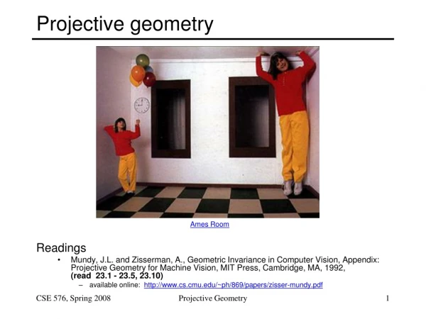
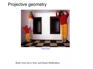
Do parallel lines intersect? Perhaps!
Fifth Euclid's postulate • For any line L and a point P not on L, there exists a unique line that is parallel to L (never meets L) and passes through P. • At first glance it would seem that the parallel postulate ought to be a theorem deducible from the other more basic postulates. • For centuries mathematicians tried to prove it. • Eventually it was discovered that the parallel postulate is logically independent of the other postulates, and you get a perfectly consistent system even if you assume that parallel postulate is false.
Alternative postulates • Non-Euclidean geometry; though not a typical one • The projective axiom: Any two lines intersect (in exactly one point). • More intuitive approach:Take each line of ordinary Euclidean geometry and add to it one extra object called a point at infinity. In addition, the collection of all the extra objects together is also called a line in projective plane (called the line at infinity).
Why Projective Geometry? • A more appropriate framework when dealing with projection related issues. • Perspective projection: Photophraphy Human vision • Perspective projection is a non-linear mapping with Euclidean coordinates, but a linear mapping with homogeneous coordinates
Overview • 2D Projective Geometry • 3D Projective Geometry • Application: Invariant matching • From 2D images to 3D space
Homogeneous representation of points on if and only if Homogeneous coordinates but only 2DOF Inhomogeneous coordinates Homogeneous coordinates Homogeneous representation of lines equivalence class of vectors, any vector is representative Set of all equivalence classes in R3(0,0,0)T forms P2 The point x lies on the line l if and only if xTl=lTx=0
Line joining two points The line through two points and is Points from lines and vice-versa Intersections of lines The intersection of two lines and is Example
tangent vector normal direction Example Ideal points Line at infinity Ideal points and the line at infinity Intersections of parallel lines Note that in P2 there is no distinction between ideal points and others
A model for the projective plane exactly one line through two points exaclty one point at intersection of two lines
Duality principle: To any theorem of 2-dimensional projective geometry there corresponds a dual theorem, which may be derived by interchanging the role of points and lines in the original theorem. For instance, the basic axiom that "for any two points, there is a unique line that intersects both those points", when turned around, becomes "for any two lines, there is a unique point that intersects (i.e., lies on) both those lines" Duality In projective geometry, points and lines are completely interchangeable!
or homogenized or in matrix form with Conics Curve described by 2nd-degree equation in the plane 5DOF: 6 parameters
or stacking constraints yields Five points define a conic For each point the conic passes through
Theorem: A mapping h:P2P2is a projectivity if and only if there exist a non-singular 3x3 matrixH such that for any point in P2 reprented by a vector x it is true that h(x)=Hx Definition: Projective transformation or 8DOF Projective transformations Definition: A projectivity is an invertible mapping h from P2 to itself such that three points x1,x2,x3lie on the same line if and only if h(x1),h(x2),h(x3) do. projectivity=collineation=projective transformation=homography
Mapping between planes central projection may be expressed by x’=Hx (application of theorem)
Removing projective distortion select four points in a plane with know coordinates (linear in hij) (2 constraints/point, 8DOF 4 points needed) Remark: no calibration at all necessary, better ways to compute
Transformation for conics Transformation of lines and conics For a point transformation Transformation for lines
A hierarchy of transformations Projective linear group Affine group (last row (0,0,1)) Euclidean group (upper left 2x2 orthogonal) Oriented Euclidean group (upper left 2x2 det 1) Alternative, characterize transformation in terms of elements or quantities that are preserved or invariant e.g. Euclidean transformations leave distances unchanged
orientation preserving: orientation reversing: Class I: Isometries (iso=same, metric=measure) 3DOF (1 rotation, 2 translation) special cases: pure rotation, pure translation Invariants: length, angle, area
Class II: Similarities (isometry + scale) 4DOF (1 scale, 1 rotation, 2 translation) also know as equi-form (shape preserving) metric structure = structure up to similarity (in literature) Invariants: ratios of length, angle, ratios of areas, parallel lines
Class III: Affine transformations 6DOF (2 scale, 2 rotation, 2 translation) non-isotropic scaling! (2DOF: scale ratio and orientation) Invariants: parallel lines, ratios of parallel lengths, ratios of areas
Class VI: Projective transformations 8DOF (2 scale, 2 rotation, 2 translation, 2 line at infinity) Action non-homogeneous over the plane Invariants: cross-ratio of four points on a line ratio of ratio of area
Action of affinities and projectivitieson line at infinity Line at infinity stays at infinity, but points move along line Line at infinity becomes finite, allows to observe vanishing points, horizon,
Decomposition of projective transformations decomposition unique (if chosen s>0) upper-triangular, Example:
Overview transformations Concurrency, collinearity, order of contact (intersection, tangency, inflection, etc.), cross ratio Projective 8dof Parallellism, ratio of areas, ratio of lengths on parallel lines (e.g midpoints), linear combinations of vectors (centroids). The line at infinity l∞ Affine 6dof Ratios of lengths, angles. The circular points I,J Similarity 4dof Euclidean 3dof lengths, areas.
Number of invariants? The number of functional invariants is equal to, or greater than, the number of degrees of freedom of the configuration less the number of degrees of freedom of the transformation e.g. configuration of 4 points in general position has 8 dof (2/pt) and so 4 similarity, 2 affinity and zero projective invariants
Projective geometry of 1D 3DOF (2x2-1) The cross ratio Invariant under projective transformations
Projective 3D Geometry • Points, lines, planes and quadrics • Transformations • П∞, ω∞and Ω ∞
3D points 3D point in R3 in P3 projective transformation (4x4-1=15 dof)
Transformation Euclidean representation Planes 3D plane Dual: points ↔ planes, lines ↔ lines
(solve as right nullspace of ) Planes from points Or implicitly from coplanarity condition
(solve as right nullspace of ) Points from planes Representing a plane by its span
Lines (4dof) Example: X-axis
Hierarchy of transformations Projective 15dof Intersection and tangency Parallellism of planes, Volume ratios, centroids, The plane at infinity π∞ Affine 12dof Similarity 7dof The absolute conic Ω∞ Euclidean 6dof Volume
The plane at infinity The plane at infinity π is a fixed plane under a projective transformation H iff H is an affinity • canonical position • contains directions • two planes are parallel line of intersection in π∞ • line // line (or plane) point of intersection in π∞
How to define an invariant 2D identifier patch on an image? • Consider a multilateral identifier patch. • Lines are invariant under the perspective projection. • 3 (4) reference points are required to obtain an affine (projective) invariant representation of the multilateral identifier patch. • Weak-perspective/perspective camera models.
R3 R2 R1 X A Affine invariant representation of a planar point • Three reference points. • Ratio of areas are invariant. • X at intersection of R1R2 and R3A. • (r1,r2) invariants defined by:
R3 R2 R1 X R4 A Projective invariant representation of a planar point • Four reference points. • Ratio of ratio of areas are invariant. • X at intersection of R1R4 and R3A. • (r1,r2) invariants defined by:
R3 A R2 R1 Affine invariant parallelogram:Three reference points Select A to make a parallelogram with three reference points R1, R2, and R3
R3 A B2 B1 R2 R1 Affine invariant parallelogram:Construction of identifier patch (1) Select B1 on R2R3
R3 B2 C2 C1 B1 R1 Affine invariant parallelogram:Construction of identifier patch (2) Select C1 on B1R1
R3 D2 C2 C1 D1 R1 Affine invariant parallelogram:Construction of identifier patch (3) Select D1 on C1R1
p1 p3 p2 q1 p4 q2 q3 q4 q5 Focal point p5 q6 p6 Image plane Perspective projection • Perspective projection of 6 (feature) points from 3D world (dorsal fin) to 2D image: pi=(xi,yi,zi) qi=(ui,vi) i=1,…,6
3D and 2D Projective Invariants • I1, I2, and I3 are 3D projective invariants (under PGL(4)). • i1, i2, i3, and i4 are 2D projective invariants (under PGL(3)). • There is no general case view-invariant. • 2D invariants impose constraints (in the form of polynomial relations) on 3D invariants. * PGL(n): Projective General Linear group of order n.