Applied Econometrics
Applied Econometrics. 11. Asymptotic Distribution Theory. Preliminary. This and our class presentation will be a moderately detailed sketch of these results. More complete presentations appear in Chapter 4 of your text. Please read this chapter thoroughly. We will develop the results that we

Applied Econometrics
E N D
Presentation Transcript
1. Applied Econometrics William Greene
Department of Economics
Stern School of Business
2. Applied Econometrics 11. Asymptotic Distribution Theory
3. Preliminary This and our class presentation will be a moderately detailed sketch of these results. More complete presentations appear in Chapter 4 of your text. Please read this chapter thoroughly. We will develop the results that we need as we proceed. Also, (I believe) that this topic is the most difficult conceptually in this course, so do feel free to ask questions in class.
4. Asymptotics: Setting Most modeling situations involve stochastic regressors, nonlinear models or nonlinear estimation techniques. The number of exact statistical results, such as expected value or true distribution, that can be obtained in these cases is very low. We rely, instead, on approximate results that are based on what we know about the behavior of certain statistics in large samples. Example from basic statistics: What can we say about 1/ We know a lot about . What do we know about its reciprocal?
5. Convergence Definitions, kinds of convergence as n grows large:
1. To a constant; example, the sample mean,
2. To a random variable; example, a t statistic with n -1 degrees of freedom
6. Convergence to a Constant Sequences and limits.
Sequence of constants, indexed by n
(n(n+1)/2 + 3n + 5)
Ordinary limit: -------------------------- ? ?
(n2 + 2n + 1)
(The use of the �leading term�)
Convergence of a random variable. What does it mean for a random variable to converge to a constant? Convergence of the variance to zero. The random variable converges to something that is not random.
7. Convergence Results Convergence of a sequence of random variables to a constant - convergence in mean square: Mean converges to a constant, variance converges to zero. (Far from the most general, but definitely sufficient for our purposes.)
A convergence theorem for sample moments. Sample moments converge in probability to their population counterparts.
Generally the form of The Law of Large Numbers. (Many forms; see Appendix D in your text.)
Note the great generality of the preceding result. (1/n)Sig(zi) converges to E[g(zi)].
8. Probability Limit
9. Mean Square Convergence
10. Probability Limits and Expecations
What is the difference between
E[xn] and plim xn?
11. Consistency of an Estimator If the random variable in question, xn is an estimator (such as the mean), and if
plim xn = ?
Then xn is a consistent estimator of ?.
Estimators can be inconsistent for two reasons:
(1) They are consistent for something other than the thing that interests us.
(2) They do not converge to constants. They are not consistent estimators of anything.
We will study examples of both.
12. The Slutsky Theorem Assumptions: If
xn is a random variable such that plim xn = ?.
For now, we assume ? is a constant.
g(.) is a continuous function with continuous derivatives. g(.) is not a function of n.
Conclusion: Then plim[g(xn)] = g[plim(xn)] assuming g[plim(xn)] exists. (VVIR!)
Works for probability limits. Does not work for expectations.
13. Slutsky Corollaries
14. Slutsky Results for Matrices Functions of matrices are continuous functions of the elements of the matrices. Therefore,
If plimAn = A and plimBn = B (element by element), then
Plim(An-1) = [plim An]-1 = A-1
and
plim(AnBn) = plimAnplim Bn = AB
15. Limiting Distributions Convergence to a kind of random variable instead of to a constant
xn is a random sequence with cdf Fn(xn). If plim xn = ? (a constant), then Fn(xn) becomes a point. But, Fn may converge to a specific random variable. The distribution of that random variable is the limiting distribution of xn.
16. Limiting Distribution
17. A Slutsky Theorem for Random Variables (Continuous Mapping)
18. An Extension of the Slutsky Theorem
19. Application of the Slutsky Theorem
20. Central Limit Theorems Central Limit Theorems describe the large sample behavior of random variables that involve sums of variables. �Tendency toward normality.�
Generality: When you find sums of random variables, the CLT shows up eventually.
The CLT does not state that means of samples have normal distributions.
21. A Central Limit Theorem
22. Lindberg-Levy vs. Lindeberg-Feller Lindeberg-Levy assumes random sampling � observations have the same mean and same variance.
Lindeberg-Feller allows variances to differ across observations, with some necessary assumptions about how they vary.
Most econometric estimators require Lindeberg-Feller.
23. Order of a Sequence Order of a sequence
�Little oh� o(.). Sequence hn is o(n?) (order less than n?) iff n-? hn ? 0.
Example: hn = n1.4 is o(n1.5) since n-1.5 hn = 1 /n.1 ? 0.
�Big oh� O(.). Sequence hn is O(n?) iff n-? hn ? a finite nonzero constant.
Example 1: hn = (n2 + 2n + 1) is O(n2).
Example 2: ?ixi2 is usually O(n1) since this is n?the mean of xi2
and the mean of xi2 generally converges to E[xi2], a finite
constant.
What if the sequence is a random variable? The order is in terms of the variance.
Example: What is the order of the sequence in random sampling?
Var[ ] = s2/n which is O(1/n)
24. Asymptotic Distribution An asymptotic distribution is a finite sample approximation to the true distribution of a random variable that is good for large samples, but not necessarily for small samples.
Stabilizing transformation to obtain a limiting distribution. Multiply random variable xn by some power, a, of n such that the limiting distribution of naxn has a finite, nonzero variance.
Example, has a limiting variance of zero, since the variance is s2/n. But,
the variance of vn is s2. However, this does not stabilize the distribution because E[ ] = v n�.
The stabilizing transformation would be
25. Asymptotic Distribution Obtaining an asymptotic distribution from a limiting distribution
Obtain the limiting distribution via a stabilizing transformation
Assume the limiting distribution applies reasonably well in
finite samples
Invert the stabilizing transformation to obtain the asymptotic
distribution
Asymptotic normality of a distribution.
26. Asymptotic Efficiency Comparison of asymptotic variances
How to compare consistent estimators? If both converge to constants, both variances go to zero.
Example: Random sampling from the normal distribution,
Sample mean is asymptotically normal[�,s2/n]
Median is asymptotically normal [�,(p/2)s2/n]
Mean is asymptotically more efficient
27. The Delta Method The delta method (combines most of these concepts)
Nonlinear transformation of a random variable: f(xn) such that
plim xn = ? but ?n (xn - ?) is asymptotically normally
distributed. What is the asymptotic behavior of f(xn)?
Taylor series approximation: f(xn) ? f(?) + f?(?) (xn - ?)
By Slutsky theorem, plim f(xn) = f(?)
?n[f(xn) - f(?)] ? f?(?) [?n (xn - ?)]
Large sample behaviors of the LHS and RHS sides are the same (generally - requires f(.) to be nicely behaved. RHS is a constant times something familiar.
Large sample variance is [f?(?)]2 times large sample Var[?n (xn - ?)]
Return to asymptotic variance of xn
Gives us the VIR for the asymptotic distribution of a function.
28. Delta Method
29. Delta Method - Applications
30. Krinsky and Robb vs. the Delta Method
31. Delta Method � More than One Parameter
32. Log Income Equation
33. Age-Income Profile: Married=1, Kids=1, Educ=12, Female=1
34. Application: Maximum of a Function
35. Delta Method
36. Delta Method Results
37. Krinsky and Robb
38. More than One Function and More than One Coefficient
39. Application: CES Function
40. Application: CES Function
41. Application: CES Function Using Christensen and Greene Electricity data
Create ;x1=1 ;x2=logfuel ; x3=logcap ; x4=-.5*(logfuel-logcap)^2$
Regress ;lhs=logq;rh1=x1,x2,x3,x4$
Calc ;b1=b(1);b2=b(2);b3=b(3);b4=b(4) $
Calc ;gamma=exp(b1) ; delta=b2/(b2+b3) ; nu=b2+b3
; rho=b4*(b2+b3)/(b2*b3)$
Calc ;g11=exp(b1) ;g12=0 ;g13=0 ;g14=0
;g21=0 ;g22=b3/(b2+b3)^2 ;g23=-b2/(b2+b3)^2 ;g24=0
;g31=0 ;g32=1 ;g33=1 ;g34=0
;g41=0 ;g42=-b3*b4/(b2^2*b3) ;g43=-b2*b4/(b2*b3^2)
;g44=(b2+b3)/(b2*b3)$
Matrix ; g=[g11,g12,g13,g14/g21,g22,g23,g24/g31,g32,g33,g34/g41,g42,g43,g44]$
Matrix ; VDelta=G*VARB*G' $
Matrix ; theta=[gamma/delta/nu/rho] ; Stat(theta,vdelta)$
42. Estimated CES Function
43. Asymptotics for Least Squares Looking Ahead�
Assumptions: Convergence of X?X/n (doesn�t require nonstochastic or stochastic X).
Convergence of X�?/n to 0. Sufficient for consistency.
Assumptions: Convergence of (1/?n)X�? to a normal vector, gives asymptotic normality
What about asymptotic efficiency?
44. The Original IBM SSP RNG GENERATE A UNIFORMLY DISTRIBUTED RANDOM NUMBER
D2P31M = 2147483647.D0 = 231 - 1
D2P31 = 2147483655.D0 = 231 + 7
D7P5 = 16807.D0 = 75
SEED=DMOD(D7P5*SEED,D2P31M)
X= SEED/D2P31