Download
1 / 32
320 likes | 528 Views
High-Z Supernovae: The Evidence for An Accelerating Universe. R. Mutel Departmental Astrophysics Seminar February 19, 2003. Outline. Synopsis of 20 th Century Cosmology (Chronology) High-z Supernovae and the Accelerating Universe Potential problems: evolution, dust, lensing

E N D
High-Z Supernovae: The Evidence for An Accelerating Universe R. Mutel Departmental Astrophysics Seminar February 19, 2003
Outline • Synopsis of 20th Century Cosmology (Chronology) • High-z Supernovae and the Accelerating Universe • Potential problems: evolution, dust, lensing • Dark Matter update: role of ancient White dwarfs? • Latest results from WMAP – all cosmological parameters determined! • Heretical view: Burbidge’s QSSC
Brief history of Cosmological Models: pre-1980’s • 1917 – Einstein’s General Relativity: static cosmological model with ‘cosmological constant’ . Einstein assumed static Universe, needed small o > 0 to prevent collapse. • 1930 – Hubble finds Universe is expanding, Einstein drops need for (‘biggest blunder of my life’). • 1948 – QED predicts non-zero vacuum energy. Casimir effect provides experimental verification. Calculation implies ~10120o! • 1950’s Development of Steady State Model: mean density constant – expanding vacuum creates matter. Time invariance. Cosmol. constant = 0. • 1965 – Discovery of microwave cosmic background radiation (CBR), development of Big Bang cosmology. Provides natural explanation for expansion. • 1980’s – CBR too uniform (T/T < 10-4) – solved by inflation (Guth 1980). This requires a ‘flat’ Universe (tot = 1) • Early 1980’s – Observations of ordinary (luminous) matter find LM << crit (tot << 1), i.e. ‘open Universe’ geometry.
Brief history of Cosmological Models: 1980’s-1990’s • 1980’s – Rotation curves of galaxies, clusters require most gravitational mass reside in ‘dark matter’ component • 1990’s – Refined observations find LM ~ 0.02- 0.04 , CDM ~ 0.2-0.4: If tot = 1, where is the rest? • 1992 – COBE First comprehensive measurements of T/T ~3·10-5 on angular scale 6° • 1998 – First results for high-Z Type Ia SN show evidence for acceleration: explained by ‘dark energy’ (‘quintessence’) • late-1990’s – MACHO, OGLE, etc. micro-lensing surveys find microlensed events consistent with compact sub-stellar halo objects, total ~ 0.2-0.4. • 1999 – Hubble Key Project for nearby galaxies: Ho = 73 ± 6 km/s/Mpc. Standard Friedmann cosmo. Model predicts Universe’s age t = 2/3 H0-1 = 10 ± 0.8 Gyr. • 2000 – Refined measurements of stellar ages in GC (using distances from HIPPARCOS) find oldest stars are 13.4 ± 2.2 Gyr, in conflict with Ho measurements: Crisis!
Brief history of Cosmological Models late-1990’s-present • 2001 – Discovery of extremely cool (old) WD’s. Tentative density WD 0.1 CDM. • 2001-2002 – More high-z Type Ia SN enhance claims for acceleration at z<1. • 2002 – Highest redshift SN discovered on Hubble Deep Field (z~1.7, SN1997ff). Mag. Confused by lensing? • Feb 2003 – WMAP results – acoustic modes in CBR confirmed, finds tot = 1.02 ± 0.02, with =0.73 ±0.04!
Standard model: distance scale factor Ho = 65 km/s/Mpc = 0 (green), 1 (black), 2 (red)
SN1994D, A prototypical Type Ia SN • Host galaxy NGC4526, Hubble type S0, member of Virgo Cluster (15 Mpc) • Vmin =
Hubble diagram of Type Ia Supernovae. The upper panel shows the classical Hubble diagram with distance modulus vs. redshift. All data have been normalized to the m15 method. Lines of four cosmological models are drawn: full line for an empty universe ( M = 0, = 0), long-dashes for an Einstein-de Sitter model ( M = 1, = 0), dashed line for an universe dominated by the vacuum ( M = 0, = 1), and the dotted line for a flat universe ( M = 0.3, = 0.7). The lower panels are normalized to an empty universe and show the data of the High-z SN Search Team (filled squares; Riess et al. 1998) and the Supernova Cosmology Project (open squares; Perlmutter et al. 1999a).
Using distances to fit for , M 1. Observed flux, assumed luminosity of Type Ia SN are used to determine the luminosity distance: 2. From GR model, luminosity distance can be calculated as a function of , M Where:
Adding CBR results Resulting , M plot
Potential Problems with interpreting Type Ia SN Observations • Evolutionary effects in SN and/or host galaxy • Could SN Ia at z=0.5 (5 Gyr look-back time) be intrinsically fainter than at present? • Effect would have to change luminosity-light curve half-width relationship • Models at solar metallicity and 1/3 solar metallicity show only small (1%) differences in the relevant passbands
Variation in luminosity of nearby Type Ia SN over a wide range of Hubble type (and metallicity ) show little spread after MLCS correction)
Host environment, evolutionary effects continued Also, little variation in SN luminosity vs. host galaxy color: Or distance from host center
None yet, but spectra of high-z SN are difficult to measure with high SNR Are there spectral differences in low, high-z Type Ia SN?
Problems, continued • Extinction by dust • Ordinary dust: Reddening, measured by E(B-V), is consistent for low-z high-z SN. This implies IG dust must be grey. • Gray dust: Intergalactic graphitewhiskers (1µ), with density ~10-5 could cause 0.25 mag extinction at 5 Gpc, with only small amt of extinction (but one SN at z~1.7 has insufficient reddening, 2.5)
Problems, continued • Gravitational Lensing • Lenses most often dim distant objects (although integral effect is 1.0x). • For z=0.5 and M~0.5, effect is 2%, much too low to explain observed 25% dimming • This will be more important for higher-z SN surveys
Dark Matter • Rotation curve obs => CDM ~ 10-2 M/pc3
CDM densities • Central density appears to be independent of scale, from dwarf galaxies to clusters • ctr ~ 10-2 Msun pc-3 • Model Radial profile CDM r-1 (cusp at center) • CDM ~ 0.2
Dark Matter: Very cool (old) White Dwarfs? • Indirect evidence for the `dark matter' being comprised of cool white dwarfs first came from the MACHO (MAssive Compact Halo Object) gravitational microlensing experiment. • The MACHO project monitored ten million stars in the Magellanic Clouds in the hope of detecting the occasional brightening caused by a dark Halo object moving across our line of sight to one of the stars. • Microlensing experiments suggested the existence of a large number of dark objects in the Halo of our Galaxy with masses about half that of our Sun. The likely candidates for these invisible objects are distant, faint, cool white dwarfs. • However as such objects had never actually been seen before there was some doubt as to their nature. The MACHO results suggest that these stars are very numerous, and could contribute approximately 50% of the total mass of the Galaxy. WD0346+246 (V=19.1, µ = 1.3''/yr, T=3,500K)
Survey of nearby cool WD’s (Ibata et al 2001) • Survey covered of 28° x 28° • Looked for cool, faint stars with high proper motion • Complete to R=19, d = 33pc • Two detections
Several new cool WD discoveries (Scholz et al. 2002)
Using WMAP angular spectrum to determine curvature: Result is =1.02 ± 0.02 (flat) Angular scale for acoustic peaks are determined by density, ratio of electrons/photons, and distribution of dark matter at 300,000 yr. For flat Universe, first peak is expected at ~ 1 deg If the curvature is k<0 (open), ‘frozen out’ sonic density waves if a given physical wavelength appear at smaller angular scales w.r.t flat model
Using CBR spectrum to measure Electron/photon ratio at Decoupling Increasing the ratio of electrons to photons also has the effect of decreasing the sound speed of the fluid. Since the fluid moves more slowly, the secondary oscillations occur at larger angular scales. This effect shifts the location of the latter peaks in the fluctuation spectrum. WMAP: Baryon density n = (2.5 ± 0.1)·10-7 cm-3
The cosmic background radiation propagating from the surface of last scatter to is also affected by gravitational fluctuations along its path. Photons falling into the gravitational potential wells of clusters gain energy. They lose this energy when they climb out of the potential wells. If the universe is flat and composed entirely of matter, then these two effects cancel exactly and the matter along the photon path has no net gravitational effect. • If there is a cosmological constant, then the depth of gravitational potential wells decay with time. Thus, a photon which falls into a deep potential well gets to climb out of a slightly shallower well. The net effect leads to a slight increase in photon energy along this path. Another photon which travels through a low density region (which produces a potential "hill") will lose energy as it gets to descend down a shallower hill than it climbed up. • Because of this effect, a model with a cosmological constant will have additional fluctuations on large angular scales. Large angular scale measurements are most sensitive to variations in the gravitational potential at low red shift. Using CBR spectrum to Measure Cosmological Constant