Introduction to Classification and Machine Learning
740 likes | 774 Views
This text provides an overview of classification and machine learning, including topics such as supervised learning, evolutionary computation, artificial neural networks, and support vector machines. It explains the classification problem, the types of data needed, and the concept of a class attribute. The text also introduces evolutionary computation and genetic algorithms as problem-solving approaches.

Introduction to Classification and Machine Learning
E N D
Presentation Transcript
CCEB Supervised LearningEvolutionary ComputationArtificial Neural NetworksSupport Vector Machines John H. Holmes, Ph.D. Center for Clinical Epidemiology and Biostatistics University of Pennsylvania School of Medicine
What’s on the agenda for today • Review of classification • Introduction to machine learning • Evolutionary Computation • Artificial neural networks • Support vector machines
The Classification Problem A+ A- Find surface to best separate two classes.
To do classification or prediction, you need to have the right data • Pool of data • Training data • Testing data • A class attribute • Categories must be mutually exclusive • Predictor attributes
What is a class? • Defines or partitions a relation • May be dichotomous or polytomous • Is not continuous • Examples • Clinical status (Ill/Well, Dead/Alive) • Biological classification (varieties of genus, species, or order)
Mining class comparisons • Goal: to discover descriptions in the data that distinguish one class from another • These descriptions are concepts! • Data in the classes must be comparable • Same attributes • Same value-system for each attribute • Same dimensions
Some mechanistic details… • Training • Phase during which a system is trained • Focus on generalization • Testing • Phase during which a system is tested on novel cases
Instance-based learning • Testing cases (unknown class) are compared to training cases, one at a time • The training case closest to the testing case is used to output a predicted class for the testing case • You need a distance function • Euclidean most common • Compares differences between sums of squares for each attribute-value pair • Manhattan distance • Compares differences between each attribute-value pair, without squaring
A brief history of evolutionary computation 50s: Interest in evolution as a computational construct Use operators from natural genetic variation and natural selection to “evolve” solutions to problems 60s: “Evolution strategies” (Rechenberg) Applied to optimization of real-valued parameters 60s-70s: “Evolutionary programming” Genetic operators applied to finite state machines to identify candidate solutions in a solution space
So what about genetic algorithms? John Holland invented the GA in the 60s Goal: use the paradigm of natural adaptation as a general problem-solving approach Essential characteristics Population of “individuals” Represented as “chromosomes” consisting of “genes” Fitness Operators Reproduction Crossover Mutation
And why would evolution be a reasonable paradigm for solving problems? Evolution as search What is the problem space? What is the solution space? Evolution as adaptation Constantly changing problem spaces are, well, problematic! One solution at one point in time might not work in the future Evolution as a body of metarules Simplicity is the key, even as complex problems and solutions emerge
So…Genetic Algorithms Population-based technique for discovery of knowledge structures Based on idea that evolution represents search for optimum solution set Massively parallel
The vocabulary of GAs Population Set of individuals, each represented by one or more strings of characters Chromosome The string representing an individual
The vocabulary of GAs, contd. Gene The basic informational unit on a chromosome Allele The value of a specific gene Locus The ordinal place on a chromosome where a specific gene is found
Genetic operators Reproduction Increase representations of strong individuals Crossover Explore the search space Mutation Recapture “lost” genes due to crossover
GAs rely on the concept of “fitness” Ability of an individual to survive into the next generation “Survival of the fittest” Usually calculated in terms of an objective fitness function Maximization Minimization Other functions
A fitness function example: Maximize a real-valued function f(y)=y+|sin(32y)|, 0 yp Candidate solutions: all values of y in the domain Representation: Bit string: y is translated into a string of 0s and 1s representing the value of y in binary (y=12: 0011) Real number How “fit” would the value 85 be, compared to 32? ATTCGCGCCCGGGATATT Candidate solutions: all strings with legal amino acid values Representation: Translate the sequence into potential energy, if the sequence were folded into a protein The lower the potential energy, the higher the fitness
The pseudocode for a GA Initialize a population P of n chromosomes of length l Evaluate fitness F of each chromosome in the population Repeat Select two chromosomes (“parents”) proportional to their fitness With probability , apply crossover operator to create two new chromosomes (“offspring”) With probability , mutate each locus on each offspring chromosome Insert offspring into P Delete two chromosomes from P proportional to fitness Evaluate population fitness FP Until Termination condition is met (defined by target fitness function) Return final population PFinalas the set of best (most “fit”) chromosomes Each iteration is a generation, and the set of generations required to reach the final population is an epoch.
How do you select chromosomes for reproduction or deletion? Deterministic The two best (worst) chromosomes are selected for reproduction (deletion) Probabilistic Weighted roulette wheel Determine population fitness, FP Calculate each chromosome’s contribution to FP “Spin the wheel” The chromosome with the highest contribution is most likely to be selected
What are some typical parameters? Population size Depends on the complexity of the problem and l Chromosome length (l) Determined by number of variables and encoding Crossover rate () Usually 0.6-0.8 Mutation rate () Usually small, <0.001
Who will mate? Chromosomes 2 and 4, most likely! 11000 10011 11011 10000 Mutation at Locus 4 11001 10000 Crossover at Locus 2 No mutation Who will be deleted? • Chromosomes 1 and 3!
Who will mate this generation? Chromosomes 1 and 4, most likely, but the wheel says…. 1 and 2! 11001 10101 10101 11001 No mutation 10101 11001 Crossover at Locus 4 No mutation Who will be deleted? • Chromosomes 2 and 3!
Who will mate this generation? Chromosomes 1 and 4, most likely, but the wheel says…. 3 and 4! 11001 10011 11001 10011 No mutation 11001 10111 Crossover at Locus 1 Mutation at locus 3 Who will be deleted? • Chromosomes 1 and 2!
Who will mate this generation? Chromosomes 1 and 2, most likely, and the wheel says…. 1 and 2! 11001 10111 No mutation 11111 10101 11111 10001 Crossover at Locus 2 Mutation at locus 3 Who will be deleted? • Chromosomes 3 and 4!
So how did that actually work? GAs work by discovering schemata “Building blocks” of solutions Combined and/or emphasized in parallel Good solutions tend to be made up of good schemata Combinations of bit values that confer higher fitness on the chromosomes on which they exist
Neural Networks • Set of connected input/output units • Connections have weights that indicate the strength of the link between their units (neurons) • Neural networks learn by adjusting the connection weights as a result of exposure to training cases Methods: Backpropagation, self-organization
A Simple Neural Network Hidden layer Inputs Output x1 (Bitten) x2 (Rabies present) Treat Yes/No x3 (Animal captured) x4 (Animal vaccinated)
Characteristics of neural networks • Neurons are all-or-none devices • Firing depends on reaching some threshold • Networks rely on connections made between axons and dendrites • Synapses • Neurotransmitters • “Wiring”
Neuronal structure and function • Input • Always 0 or 1, until multiplied by a: • Weight • Determines a neuron’s effect on another in a connection • Inputs multiplied by their weights are processed by an: • Adder • Sums the weighted inputs from all connected neurons for processing through a: • Threshold function • Determines the output of the neuron based on the summed, weighted inputs
Weight and threshold adjustment in perceptrons • Adjustments are made only when an error occurs in the output • Weight adjustment wi(t+1)=wi(t)+wi(t) where wi(t)=(D-0)Ii
Weight and threshold adjustment in perceptrons, contd. • Threshold adjustment i(t+1)=i(t)+i(t) where i(t)=(D-0)
How the adjustment works... • If output O is correct, no change is made • If a false positive error • Each weight is adjusted by subtracting the corresponding value in the input pattern • Threshold is adjusted by subtracting 1 • If a false negative error • Each weight is adjusted by adding the corresponding value in the input pattern • Threshold is adjusted by adding 1
Training a perceptron: The pseudocode Do while output incorrect For each training case x If ox incorrect (dx- ox0) If dx - ox =1 Add logic box output vector to weight vector Else Subtract logic box output vector from weight vector x=x+1 EndDo
Backpropagation • Most common implementation of neural nets • Two-stage process • feed-forward activation from input to output layer • propagation of errors in the output backward to the input layer • Change w in proportion to the effect on the error observed at the outputs • Error=d-o • Where d=known class value, o=output from ANN
Backpropagation requires hidden layers • Middle layers build internal model of the way input patterns are related to the desired outputs • The knowledge representation is implicit in this model- it is the synapses (connectivity) that is the representation