Download
1 / 36
360 likes | 511 Views
A study of atmospheric neutrinos at India-based Neutrino Observatory. Abhijit Samanta (INO Collaboration) abhijit.samanta@saha.ac.in Saha Institue of Nuclear Physics Kolkata, India. Plan. Neutrino oscillation Neutrino parameters from present experiments INO detector

E N D
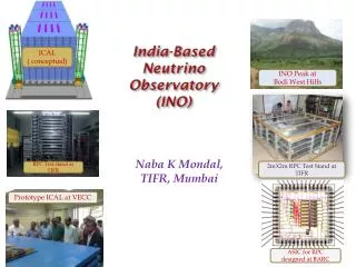
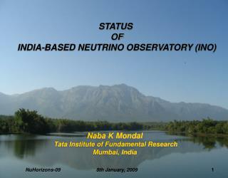
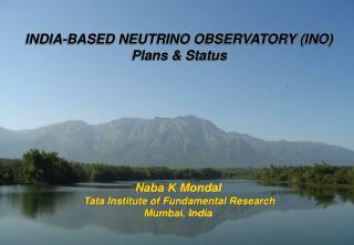
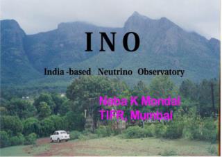
A study of atmospheric neutrinos at India-based Neutrino Observatory Abhijit Samanta (INO Collaboration) abhijit.samanta@saha.ac.in Saha Institue of Nuclear Physics Kolkata, India
Plan • Neutrino oscillation • Neutrino parameters from present experiments • INO detector • Detector simulation • Physics issues of INO: Studies with atmospherics(INO Phase I) . (Precision study of atmospheric oscillation parameters only will be discussed in details here.) Studies with beams from-decay, -factory(INO Phase II). (in short) • INO site • Conclusion
Quantum mechanics of neutrino oscillation Neutrino stationary states: |1, |2 mass m1, m2 Neutrino flavour eigenstates: |e>, | µ> Two different bases: |e =|1 cosθ +|2 sinθ |µ =-|1sinθ +|2 cosθ |e produced at t = 0 |Ψ(0) = |e = |1cos θ +|2 sinθ At a later time: |Ψ(t) = |1cos θ e-iE1t+|2 sinθe-iE2t Prob(eµ, t) = |µ |Ψ(t) |2 = 4 c2 s2 |e-iE1t - e-iE2t|2 Neutrinos are ultra-relativistic: p>>m Ei = (p2 + mi2)½ ≈ p + mi2/2p (E1 - E2)t = (m12 – m22)t /2p ≡ (∆/2p)t = L ∆/2E Prob(eµ, L) = 4 c2 s2 sin2(L/ λ) where λ = 4 E/ ∆ Survival Prob. = Prob(ee, L) = 1 - Prob(eµ, L)
Neutrino parameters frompresent experimentsNeutrinos oscillate.Neutrinos are massive and non-degenerate (m2 0) & sin2 0. • Solar m21 = 7.9 105eV2, 12 = 36o (best-fit) • Atmospheric |m322|=2 10-3eV2 , 23= 45o (best-fit) • Reactor KamLAND agrees with solar and CHOOZ constrain 1311o • Accelerator K2K confirms atmospheric results t e e e e
INO will have important role in • Confirmation of oscillation dip and rise • Sign of |m232| • Determination of 13 • CP phase • Measuring the deviation of 23 from 45o • New physics ?
Mass: 50 kTon Size : 48 m (x) 16m (y) 12 m (z) 140 layers of 6 cm thick iron with 2.5 cm gap for active elements Magnetic field ~ 1 Tesla along y-direction
Construction of RPC Two 2 mm thick float Glass Separated by 2 mm spacer 2 mm thick spacer Pickup strips Glass plates Graphite coating on the outer surfaces of glass Complete RPC
INO will have the opportunity to change the active part of the detector.
RPC Efficiency Freon 134a : 62% Argon : 30% Isobutane : 8% RPC Timing Studies Good time resolution Good up/down discrimination Bending in magnetic field can also do this job. INO prototype will be very soon at VECC, Kolkata.
Detector Simulation Package: GEANT Version : 3.2214
Track reconstruction • When a charge particle, say, ±, moves through ICAL, it gives hits(very localized electric discharge in the gases) in the active detector elements; a track in the detector. • Energy for a track can be measured in two ways: I) Energy calibration (FC only) II)curvature in a magnetic field (FC+PC). (The case I & II have been studied separately. The case I will be discussed here.) • Energy can be calibrated with number of hitsor with effective path-length (densitygeometric path). It measures the amount of energy deposited in the detector. • Angle is determined from the first few hits of the track.
Calibration of E with number of hits for a fixed zenith angle 40o Calibration of E with effective path-length for a fixed zenith angle 40o Effective path-length and number of hits are proportional to E for a fixed zenith angle.
Variation of number of hits with zenith angle for fixed E Variation of effective path-length with zenith angle for fixed E Energy calibration with effective path-length is less dependent on zenith angle than that with number of hits.
The variation of muon energy The variation of zenith angle resolution for zenith angle 54o. resolution for E= 1 GeV. (It will improve (worsen) (It will improve with increase with decrease (increase) of energy.) of zenith angle.)
Precision study with atmospheric neutrinos Event generator: NUANCE Flux : Honda Detector simulator: GEANT
Atmospheric neutrino fluxes • Low energy flux is not symmetric in up & down direction.
Oscillation of atmospheric neutrinos • L ~ 10 km for down going ~12000 km for up going • E~ few MeV-100GeV Down near detectorno oscillation Up far detector Oscillation • (Single detector with two equal sources.) up down L/E
Reduction of events (cuts) • To study the L/E resolution we generate a huge data set, say, • 83000 events in the energy range 0.8 GeV to 200 GeV with almost equal • weight up to 30GeV . • Study L/E resolutions in measured E & L/E bins. • For a particular L/E-bin, it improves with increase of E. • (With increase of E the scattering angle ( -) decreases.) • Again for a particular bin of E, resolution improves with increase of L/E. • (L resolution improves as we go far from horizon.) • Let us fix a width of the resolution as a measure of goodness. • With this criteria we find the minimum value of L/E for a given E. • We consider only longest track of an event (essentially the muon track). • No hadrons are considered a very clean signal at ICAL detector.
Reduction of events (cut) Applying the cuts defined above, we find the L/E resolutions and efficiency in neutrino (L/E – E) bins. efficiency () = (selected events)/(nuance generated events)
L/E resolution The first four figures are obtained for a bin of E & (L/E). The last figure with all E & (L/E) of 20 years un-oscillated data. The shape and width of resolution change with E & L/E . The reasons have been discussed earlier.
Taking a given year of exposure we generate a GEANT simulated data • Find up/down vs. L/E distribution (call it the “experimental data”) • Confirm oscillation with dip and then rise 5-year run Note: Efficiency must be improved if we consider zenith angle analysis for sin2 precision.
2-fit We take an event and calculate the oscillation probability P. We choose a random number X. If P > x, we keep it. Identify the resolution function from the value of E & L . If the efficiency of this bin is , smear over all L/E bins instead of smearing unity. We thus obtain a up/down plot from 20 years un-oscillated data set. We call it a“theoretical data”. If the bin size of E & L/E are made very small, we are then practically generating resolutions for every events.
Precautions in 2-fit • Up/down for plot obtained with Nuance and by random number technique from un-oscillated data as discussed above should match. • See the difference if Honda flux is with cosz bin 20 & 180 !!! • Up/down plot from random number technique matches with 180 bin of • cosz
(upper limit – lower limit) ( upper limit +lower limit) Precision = INO (with FC events only) 7 19 10-yr SKIII 10 20 10-yr MINOS 10 38 5-yr T2K 6 22 5-yr SK (present experiment) 28 39 The precision at INO will improve with inclusion of PC. Note: We use multiple resolution functions; it is for each (E L/E ) bin.
The important features of INO 1. Large mass( high statistics) magnetized Iron CALorimeter 2. Tracks are obtained from the hits (electric discharge in the gases is very transient and localized unlike Cherenkov detector) I) High angular resolution and high charge identification capability (bending of track in magnetic field) II) Good E resolution III) Good time resolution ( ~ nanosec) up/down discrimination 3. INO to CERN baseline magic baseline (degeneracy in observables due to CP-phase is negligible.) Important role in the present open issues in neutrino physics e.g., determination of mass hierarchy, 13, CP-phase search for new physics ……..
PUSHEP (Pykara Ultimate Stage Hydro Electric Project) in South India
Reduction of muon background with depth INO is in good depth !!! PUSHEPselected, after a detailed comparison with Rammam
INO Collaboration In the last year 41 Experimentalists + Engineers 22 Theorists INO is growing up rapidly through The INO training school Phase-I (April 10 – 25) at Harish-Chandra Research Institute, Allahabad on Theoretical and Phenomenological Aspects Phase-II (May 1 – 13) Saha Institute of Nuclear Physics/Variable Energy Cyclotron Centre, Kolkata on Experimental Aspects URL: http://www.imsc.res.in/ ~ino
Acknowledgement I am grateful to Dr. Michele Maltoni for arranging this talk. I want to express my gratitude to Professor Amitava Raychaudhuri, Professor Sudeb Bhattacharya and Professor Kamales Kar for all kind of supports, suggestions and discussions. I am also thankful to my collaborators Professor Ambar Ghosal and Professor Debasish Majumdar for discussions. Finally I want to acknowledge the supports from DST, India as well as from ASICTP.