Download
1 / 30
320 likes | 458 Views
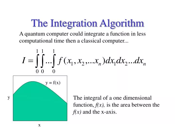
y = f(x). y. x. The Integration Algorithm. A quantum computer could integrate a function in less computational time then a classical computer... . The integral of a one dimensional function, f(x), is the area between the f(x) and the x-axis. y=f(x). y=f(x). y. y. x. x.

E N D
y = f(x) y x The Integration Algorithm A quantum computer could integrate a function in less computational time then a classical computer... The integral of a one dimensional function, f(x), is the area between the f(x) and the x-axis.
y=f(x) y=f(x) y y x x Integration via Summation The integral, I, can be approximated by a sum, S. Taking more equally spaced points in the summation, leads to a better the approximation of the integral.
y=f(x) y x Summation We first evaluate the sum where M is the number of points used in the approximation. This sums the height of all the boxes. Multiplying this by the width of each box gives the area under the boxes. Defining , we see that S is equal to the average value of f(a).
Quantum Averaging The average of a function can be found on a quantum computer in the following way... Initial state of quantum computer 1 work qubit log2(M) function qubits - these qubits store the number for which we will evaluate the function, f(a).
The Hadamard Transform The Hadamard transform, H, takes a qubit from a ‘classical’ 0 or 1 state, to a superposition of 0 and 1. Hence, Hadamards on all function qubits in the initial state of our quantum computer will give an equal superposition of all possible states, a, allowing us to evaluate f(a) for all input states.
Quantum Averaging We now conditionally rotate the work qubit by an amount f(a) depending on the state of the function qubits. This puts our quantum computer into the state... If we now perform another set of Hadamards on the function qubits the state will have an amplitude of from which we can get S.
Quantum Averaging via NMR Measurement of a quantum system in a superposition state is probabilistic. Therefore, we can only extract the amplitude of a particular state by repeated experiments and measurements of the system. The more experiments the closer we can estimate the amplitude. An NMR quantum information processor allows us to read out the entire state of our system exactly - allowing us to bypass methods necessary to amplify the amplitude.
work bit Extract amplitude of evaluate f(a) state function bits H H H H H H H H Integration Gate Sequence Sequence of conditional rotations - rotate work bit by some angle if the function bit is 1.
Extract amplitude of state H H H H H H H H Integrating Sinusoidal Functions To integrate a sinusoidal function between 0 and 1 would require each state, a, to conditionally rotate the work bit by , where work bit function bits a is stored as a binary number . Thus the sequence to evaluate f(a) is a series of conditional gates that rotate the work bit by an amount .
1 0 1 Integration of Actual integration yields: The integration algorithm taking the four data points shown above yields:
1 Extract amplitude of 0 1 state H H H H conditional rotations Integrating work bit function bits
Integration Algorithm for Amplitude of state = .433 Pseudo pure state Hadamard on function bits Bits 1 and 3 are function bits. Hadamard on function bits Conditional rotation from most significant function bit Conditional rotation from least significant function bit
1 0 1 Integration of Actual integration yields: The integration algorithm taking the four data points shown above yields:
1 Extract amplitude of 1 0 state H H H H Integrating work bit function bits Controlled-NOT gate
Initial state Integration Algorithm Using CNOT CNOT31 Amplitude of state = .5 Hadamard on function bits Hadamard on function bits
JIS I S 9.6 T RF wave 2-3 Dibromothiophene Quantum Information Processing using NMR Spectrometer Nuclear Spins as qubits ADC for data acquisition RF synthesizer and amplifier Gradient control 0 1 B sample test tube wave guides RF Wave High field magnet
Internal Hamiltonian • The evolution of a spin system is generated by Hamiltonians • Internal Hamiltonian: JIS Hint=wIIz+wSSz+2pJISIzSz I S 9.6 T interaction with B field spin-spin coupling 2-3 Dibromothiophene
External Hamiltonian • Experimentally Controlled Hamiltonian: • Total Hamiltonian: Hext(t)=wRFx(t)·(Ix+Sx)+wRFy(t)·(Iy+Sy) spins couple to RF field JIS I S 9.6 T Htotal (t)= Hint + Hext(t) Htotal(t) controlled via Hext(t) RF wave 2-3 Dibromothiophene
J12= 54.1 J23= 35.0 C1 C3 C2 J13= -1.3 The Alanine Spin System
RF nutation rate (radians) time Radio Frequency Pulses RF pulses are designed to implement a single unitary operator on any number of spins. A computer program designed for the specific spin system is used to search for such a pulse based on the parameters: duration of pulse, power, phase, and frequency offset. This pulse implements a Hadamard gate on the second and third spins.
Encode Decode No Error Flip Bit 1 Flip Bit 2 Flip Bit 3 Quantum Error Correction Start with an initial state and some extra spins Single bit errors become correlated errors Measure the extra bits to collapse to one error and learn what error occurred. Then correct it. Never need to know the original state!
Encode Decode Engineered Noise Information Encoded Un-Encoded Noise strength (Hz) Decoherence Free Subspace
Weak Noise Strong Noise Limit Info No Encoding, Y Noise Un-Encoded 0.24 Z-X Noise Information NS-Encoded 0.70 No Noise Encoded, Y, Z Noise Z-X Noise 0.70 Z-Y Noise 0.70 Noise Strength (Hz) Noiseless Subsystem Experiment
Tomography Not all elements of the density matrix are observable on an NMR spectra. To observe the other elements of the density matrix requires repeating the experiment 7 times with readout pulses appended to the pulse program. This is done without changing any other parameters of the pulse program.
Creation of a Pseudo-Pure State thermal state 72o spin 2 rotation and gradient Control2 90o y on 1 & 3 Add some identity gradient Fake ‘swap’ 1 &2 Pseudo-pure state
NMR Simulation Hadamard on function bits Pseudo-pure state Hadamard on function bits Conditional rotation from most significant function bit Conditional rotation from least significant function bit Simulator correlation -.92
NMR CNOT Simulation Pseudo-pure state CNOT31 Hadamard on function bits Hadamard on function bits Simulator correlation -.99
NMR Experiment Pseudo-pure state CNOT31 projection = .98 correlation = .97 Hadamard on function bits Hadamard on function bits correlation = .92 correlation = .91
The element gives the result of the integration. element Integration Results Amplitude = .497
Conclusions • Concrete mapping between integration algorithm and NMR QIP implementation. • Sufficient control with current NMR quantum information processors to execute integration in small Hilbert spaces. • NMR QIP version of algorithm does not require amplitude amplification. • General approach for integrating sinusoidal functions.