Download
1 / 1
10 likes | 108 Views
Study on fishery model with dynamic equations, analyzing population growth, fishing effort, and optimal harvest policy with taxation control. Discussions on steady states and local stability included.

E N D
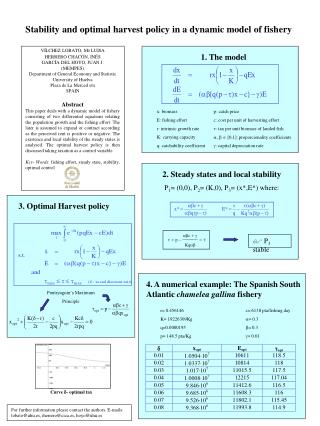
Stability and optimal harvest policy in a dynamic model of fishery VÍLCHEZ LOBATO, M0 LUISA HERRERO CHACÓN, INÉS GARCÍA DEL HOYO, JUAN J. (MEMPES) Department of General Economy and Statistic University of Huelva Plaza de La Merced s/n SPAIN Abstract This paper deals with a dynamic model of fishery consisting of two differential equations relating the population growth and the fishing effort. The later is assumed to expand or contract according as the perceived rent is positive or negative. The existence and local stability of the steady states is analysed. The optimal harvest policy is then discussed taking taxation as a control variable. Key- Words: fishing effort, steady state, stability, optimal control 1. The model x: biomass E: fishing effort r: intrinsic growth rate K: carrying capacity q: catchability coefficient p: catch price c: cost per unit of harvesting effort : tax per unit biomass of landed fish , [0,1]: proporcionality coefficients : capital depreciation rate 2. Steady states and local stability P1= (0,0), P2= (K,0), P3= (x*,E*) where: 3. Optimal Harvest policy P3 stable 4. A numerical example: The Spanish South Atlantic chamelea gallina fishery Pontryaguin’s Maximum Principle r= 0.456146 c= 6138 pta/fishing day K= 19226309Kg = 0.3 q=0.0000195 = 0.3 p= 148.5 pta/Kg = 0.01 Curve - optimal tax For further information please contact the authors. E-mails: lobato@uhu.es, iherrero@cica.es, hoyo@uhu.es