
Estimating Yield Losses from Nutrient Rate Reductions
Learn a mathematical method to estimate yield losses by reducing nutrient rates. Understand quadratic equations modeling crop responses and estimate quadratic coefficients for better farming decisions.

Estimating Yield Losses from Nutrient Rate Reductions
E N D
Presentation Transcript
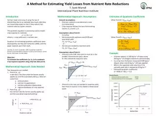
A Method for Estimating Yield Losses from Nutrient Rate ReductionsT. Scott MurrellInternational Plant Nutrition Institute Introduction Mathematical Approach: Assumptions Estimates of Quadratic Coefficients Farmers need some way of using the law ofdiminishing returns to estimate how much yield they can reasonably expect to lose if they reduce their nutrient rates by a given amount. The quadratic equation is commonly used to model crop response to nutrients: y = a + bx + cx2 where y = crop yield and x = nutrient rate. Equations for estimating quadratic coefficients were developed by van Raij and Cantarella (1996), and this paper expands upon their work.(van Raij, B. and H. Cantarella. 1996. A quadratic model for fertilizer recommendations based on results of soil analyses. Comm. Soil Sci. Plant Anal. 27:1595-1610) Objective: To estimate the coefficients (a, b, c) of a quadratic crop response equation using only two data points • General assumptions: • Only one nutrient is considered at a time(no interactions) • Crop response follows the law of diminishing returns: b> 0 and c< 0 • Assumptions about Point B:It is either • the economically optimum rate (EOR) and associated yield: (xf, yf) = (xEOR, yEOR)- or - • the rate just needed to maximize yield: (xf, yf) = (xMAX, yMAX) • Assumptions about Point A: • If Point B is the EOR, then point A must be in the shaded 2-dimensional space, whereR = the nutrient to crop price ratio: • If Point B is the rate just needed to maximize yield, then Point A must be in the shaded 2-dimensional space: When Point B = (xEOR, yEOR): When Point B = (xMAX, yMAX): (yEOR - yr – RxEOR + Rxr) c = (-xEOR2 + 2xrxEOR – xr2) b = R - 2cxEOR a = yr – Rxr + c(2xEORxr – xr2) Example • A farmer expects 12 500 kg ha-1 of maize using 200 kg ha-1 of nitrogen (maximum yield and rate) • In a strip trial, the farmer measured 8 000 kg ha-1 of grain when only 50 kg ha-1 of N was applied • What is the expected yield reduction if the normally used rate is reduced by 30 kg ha-1? • Estimated quadratic coefficients:a = 4500; b = 80; c = -0.2 (yr – ymax) y = (yEOR – RxEOR) + Rx c = (xmax – xr)2 yEOR Mathematical Approach: Data Needed Point B (xEOR, yEOR) b = -2cxmax yEOR - RxEOR Point A a = yr + c(2xrxmax – xr2) • Two data points are needed: • Point A (xr, yr):a rate that is less than what the farmer usually applies (xr) and the associated yield (yr). Data can come from: • omission plots • nutrient misapplications • soil test calibration relationships • regional databases of crop response • Point B (xf, yf):the nutrient rate the farmer usually applies (xf) and the associated expected yield (yf) y = 0 + bx + cx2 0 0 xEOR yf Point B (xf, yf) y = yMAX Yield (y) yr Point A (xr, yr) yMAX Point B (xMAX, yMAX) Point A xr xf Nutrient rate (x) y = 0 + bx + cx2 0 0 xMAX


