Download
1 / 64
650 likes | 871 Views
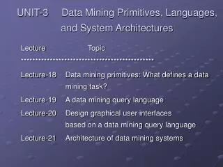
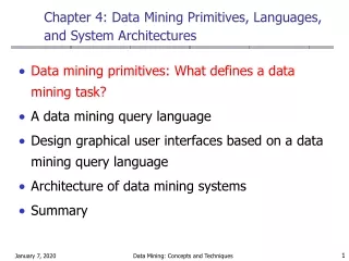
Data Mining Primitives, Languages and System Architecture. CSE 634-Datamining Concepts and Techniques Professor Anita Wasilewska Presented By Sushma Devendrappa - 105526184 Swathi Kothapalli - 105531380. Sources/References.

E N D
Data Mining Primitives, Languages and System Architecture CSE 634-Datamining Concepts and Techniques Professor Anita Wasilewska Presented By Sushma Devendrappa - 105526184 Swathi Kothapalli - 105531380
Sources/References • Data Mining Concepts and Techniques –Jiawei Han and Micheline Kamber, 2003 • Handbook of Data Mining and Discovery- Willi Klosgen and Jan M Zytkow, 2002 • Lydia: A System for Large-Scale News Analysis- String Processing and Information Retrieval: 12th International Conference, SPRING 2005, Buenos Aires, Argentina, November 2-4 2005. • Information Retrieval: Data Structures and Algorithms - W. Frakes and R. Baeza-Yates, 1992 • Geographical Information System - http://erg.usgs.gov/isb/pubs/gis_poster/
Content • Data mining primitives • Languages • System architecture • Application – Geographical information system (GIS) • Paper - Lydia: A System for Large-Scale News Analysis
Introduction • Motivation- need to extract useful information and knowledge from a large amount of data (data explosion problem) • Data Mining tools perform data analysis and may uncover important data patterns, contributing greatly to business strategies, knowledge bases, and scientific and medical research.
What is Data Mining??? • Data mining refers to extracting or “mining” knowledge from large amounts of data. Also referred as Knowledge Discovery in Databases. • It is a process of discovering interesting knowledge from large amounts of data stored either in databases, data warehouses, or other information repositories.
Graphical user interface Pattern evaluation Knowledge base Data mining engine Database or data warehouse server Data cleansing Data Integration Filtering Database Data warehouse Architecture of a typical data mining system
Misconception: Data mining systems can autonomously dig out all of the valuable knowledge from a given large database, without human intervention. If there was no user intervention then the system would uncover a large set of patterns that may even surpass the size of the database. Hence, user interference is required. This user communication with the system is provided by using a set of data mining primitives.
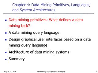
Data Mining Primitives Data mining primitives define a data mining task, which can be specified in the form of a data mining query. • Task Relevant Data • Kinds of knowledge to be mined • Background knowledge • Interestingness measure • Presentation and visualization of discovered patterns
Task relevant data • Data portion to be investigated. • Attributes of interest (relevant attributes) can be specified. • Initial data relation • Minable view
Example • If a data mining task is to study associations between items frequently purchased at AllElectronics by customers in Canada, the task relevant data can be specified by providing the following information: • Name of the database or data warehouse to be used (e.g., AllElectronics_db) • Names of the tables or data cubes containing relevant data (e.g., item, customer, purchases and items_sold) • Conditions for selecting the relevant data (e.g., retrieve data pertaining to purchases made in Canada for the current year) • The relevant attributes or dimensions (e.g., name and price from the item table and income and age from the customer table)
Kind of knowledge to be mined • It is important to specify the knowledge to be mined, as this determines the data mining function to be performed. • Kinds of knowledge include concept description, association, classification, prediction and clustering. • User can also provide pattern templates. Also called metapatterns or metarules or metaqueries.
Example A user studying the buying habits of allelectronics customers may choose to mine association rules of the form: P (X:customer,W) ^ Q (X,Y) => buys (X,Z) Meta rules such as the following can be specified: age (X, “30…..39”) ^ income (X, “40k….49K”) => buys (X, “VCR”) [2.2%, 60%] occupation (X, “student ”) ^ age (X, “20…..29”)=> buys (X, “computer”) [1.4%, 70%]
Background knowledge • It is the information about the domain to be mined • Concept hierarchy: is a powerful form of background knowledge. • Four major types of concept hierarchies: schema hierarchies set-grouping hierarchies operation-derived hierarchies rule-based hierarchies
Concept hierarchies (1) • Defines a sequence of mappings from a set of low-level concepts to higher-level (more general) concepts. • Allows data to be mined at multiple levels of abstraction. • These allow users to view data from different perspectives, allowing further insight into the relationships. • Example (location)
all Level 0 USA Level 1 Canada British Columbia Ontario New York Illinois Level 2 Level 3 Vancouver Victoria Toronto Ottawa New York Buffalo Chicago Example
Concept hierarchies (2) • Rolling Up - Generalization of data Allows to view data at more meaningful and explicit abstractions. Makes it easier to understand Compresses the data Would require fewer input/output operations • Drilling Down - Specialization of data Concept values replaced by lower level concepts • There may be more than concept hierarchy for a given attribute or dimension based on different user viewpoints • Example: Regional sales manager may prefer the previous concept hierarchy but marketing manager might prefer to see location with respect to linguistic lines in order to facilitate the distribution of commercial ads.
Schema hierarchies • Schema hierarchy is the total or partial order among attributes in the database schema. • May formally express existing semantic relationships between attributes. • Provides metadata information. • Example: location hierarchy street < city < province/state < country
Set-grouping hierarchies • Organizes values for a given attribute into groups or sets or range of values. • Total or partial order can be defined among groups. • Used to refine or enrich schema-defined hierarchies. • Typically used for small sets of object relationships. • Example: Set-grouping hierarchy for age {young, middle_aged, senior} all (age) {20….29} young {40….59} middle_aged {60….89} senior
Operation-derived hierarchies • Operation-derived: based on operations specified operations may include decoding of information-encoded strings information extraction from complex data objects data clustering Example: URL or email address xyz@cs.iitm.in gives login name < dept. < univ. < country
Rule-based hierarchies • Rule-based: Occurs when either whole or portion of a concept hierarchy is defined as a set of rules and is evaluated dynamically based on current database data and rule definition • Example: Following rules are used to categorize items as low_profit, medium_profit and high_profit_margin. low_profit_margin(X) <= price(X,P1)^cost(X,P2)^((P1-P2)<50) medium_profit_margin(X) <= price(X,P1)^cost(X,P2)^((P1-P2)≥50)^((P1-P2)≤250) high_profit_margin(X) <= price(X,P1)^cost(X,P2)^((P1-P2)>250)
Interestingness measure (1) • Used to confine the number of uninteresting patterns returned by the process. • Based on the structure of patterns and statistics underlying them. • Associate a threshold which can be controlled by the user. • patterns not meeting the threshold are not presented to the user. • Objective measures of pattern interestingness: simplicity certainty (confidence) utility (support) novelty
Interestingness measure (2) • Simplicity a patterns interestingness is based on its overall simplicity for human comprehension. Example: Rule length is a simplicity measure • Certainty (confidence) Assesses the validity or trustworthiness of a pattern. confidence is a certainty measure confidence (A=>B) = # tuples containing both A and B# tuples containing A A confidence of 85% for the rulebuys(X, “computer”)=>buys(X,“software”) means that 85% of all customers who purchased a computer also bought software
Interestingness measure (3) • Utility (support) usefulness of a pattern support (A=>B) = # tuples containing both A and Btotal # of tuples A support of 30% for the previous rule means that 30% of all customers in the computer department purchased both a computer and software. • Association rules that satisfy both the minimum confidence and support threshold are referred to as strong association rules. • Novelty Patterns contributing new information to the given pattern set are called novel patterns (example: Data exception). removing redundant patterns is a strategy for detecting novelty.
Presentation and visualization • For data mining to be effective, data mining systems should be able to display the discovered patterns in multiple forms, such as rules, tables, crosstabs (cross-tabulations), pie or bar charts, decision trees, cubes, or other visual representations. • User must be able to specify the forms of presentation to be used for displaying the discovered patterns.
Data mining query languages • Data mining language must be designed to facilitate flexible and effective knowledge discovery. • Having a query language for data mining may help standardize the development of platforms for data mining systems. • But designed a language is challenging because data mining covers a wide spectrum of tasks and each task has different requirement. • Hence, the design of a language requires deep understanding of the limitations and underlying mechanism of the various kinds of tasks.
Data mining query languages (2) • So…how would you design an efficient query language??? • Based on the primitives discussed earlier. • DMQL allows mining of different kinds of knowledge from relational databases and data warehouses at multiple levels of abstraction.
DMQL • Adopts SQL-like syntax • Hence, can be easily integrated with relational query languages • Defined in BNF grammar [ ] represents 0 or one occurrence { } represents 0 or more occurrences Words in sans serif represent keywords
DMQL-Syntax for task-relevant data specification • Names of the relevant database or data warehouse, conditions and relevant attributes or dimensions must be specified • use database ‹database_name› or use data warehouse ‹data_warehouse_name› • from ‹relation(s)/cube(s)› [where condition] • in relevance to ‹attribute_or_dimension_list› • order by ‹order_list› • group by ‹grouping_list› • having ‹condition›
Syntax for Kind of Knowledge to be Mined • Characterization : ‹Mine_Knowledge_Specification› ::= mine characteristics [as ‹pattern_name›] analyze ‹measure(s)› • Example: mine characteristics as customerPurchasing analyze count% • Discrimination: ‹Mine_Knowledge_Specification› ::= mine comparison [as ‹pattern_name›] for ‹target_class› where ‹target_condition›{versus ‹contrast_class_i where ‹contrast_condition_i›} analyze ‹measure(s)› • Example: Mine comparison as purchaseGroups for bigspenders where avg(I.price) >= $100 versus budgetspenders where avg(I.price) < $100 analyze count
Syntax for Kind of Knowledge to be Mined (2) • Association: ‹Mine_Knowledge_Specification› ::= mine associations [as ‹pattern_name›] [matching ‹metapattern›] • Example: mine associations as buyingHabits matching P(X: customer, W) ^ Q(X,Y) => buys (X,Z) • Classification: ‹Mine_Knowledge_Specification› ::= mine classification [as‹pattern_name›] analyze‹classifying_attribute_or_dimension› • Example: mine classification as classifyCustomerCreditRating analyze credit_rating
Syntax for concept hierarchy specification • More than one concept per attribute can be specified • Use hierarchy ‹hierarchy_name› for ‹attribute_or_dimension› • Examples: Schemaconcept hierarchy (ordering is important) • define hierarchy location_hierarchy on address as [street,city,province_or_state,country] Set-Grouping concept hierarchy • define hierarchy age_hierarchy for age on customer as level1: {young, middle_aged, senior} < level0: all level2: {20, ..., 39} < level1: young level2: {40, ..., 59} < level1: middle_aged level2: {60, ..., 89} < level1: senior
Syntax for concept hierarchy specification (2) • operation-derived concept hierarchy • define hierarchy age_hierarchyfor age on customer as {age_category(1), ..., age_category(5)} := cluster (default, age, 5) < all(age) • rule-based concept hierarchy • define hierarchy profit_margin_hierarchy on itemas level_1: low_profit_margin < level_0: all if (price - cost)< $50 level_1: medium-profit_margin < level_0: all if ((price - cost) > $50) and ((price - cost) <= $250)) level_1: high_profit_margin < level_0: all if (price - cost) > $250
Syntax for interestingness measure specification • with [‹interest_measure_name›] threshold = ‹threshold_value› • Example: with support threshold= 5% with confidence threshold= 70%
Syntax for pattern presentation and visualization specification • display as ‹result_form› • The result form can be rules, tables, cubes, crosstabs, pie or bar charts, decision trees, curves or surfaces. • To facilitate interactive viewing at different concept levels or different angles, the following syntax is defined: ‹Multilevel_Manipulation› ::= roll up on ‹attribute_or_dimension› | drill down on ‹attribute_or_dimension› | add ‹attribute_or_dimension› | drop ‹attribute_or_dimension›
Architectures of Data Mining System • With popular and diverse application of data mining, it is expected that a good variety of data mining system will be designed and developed. • Comprehensive information processing and data analysis will be continuously and systematically surrounded by data warehouse and databases. • A critical question in design is whether we should integrate data mining systems with database systems. • This gives rise to four architecture: - No coupling - Loose Coupling - Semi-tight Coupling- Tight Coupling
Cont. • No Coupling: DM system will not utilize any functionality of a DB or DW system • Loose Coupling: DM system will use some facilities of DB and DW system like storing the data in either of DB or DW systems and using these systems for data retrieval • Semi-tight Coupling: Besides linking a DM system to a DB/DW systems, efficient implementation of a few DM primitives. • Tight Coupling: DM system is smoothly integrated with DB/DW systems. Each of these DM, DB/DW is treated as main functional component of information retrieval system.
Paper Discussion Lydia: A System for Large-Scale News Analysis Levon Lloyd, Dimitrios Kechagias, Steven Skiena Department of Computer Science State University of New York at Stony Brook Published in 12th International Conference SPRING 2005, Buenos Aires, Argentina, November 2-4 2005
Abstract • This paper is on “Text Mining” system called Lydia. • Periodical publications represent a rich and recurrent source of knowledge on both current and historical events. • The Lydia project seeks to build a relational model of people, places, and things through natural language processing of news sources and the statistical analysis of entity frequencies and co-locations. • Perhaps the most familiar news analysis system is Google News
Lydia Text Analysis System • Lydia is designed for high-speed analysis of online text • Lydia performs a variety of interesting analysis on named entities in text, breaking them down by source, location and time.
Block Diagram of Lydia System Juxtaposition Analysis Applications Synset Identification DataBase Document Extractor Heatmap Generation Syntax Tagging Actor Classification Rule Based Processing Geographic Normalization POS Tagging
Process Involved • Spidering and Article Classification • Named Entity Recognition • Juxtaposition Analysis • Co-reference Set Identification • Temporal and Spatial Analysis
News Analysis with Lydia • Juxtapositional Analysis. • Spatial Analysis • Temporal entity analysis
Juxtaposition Analysis • Mental model of where an entity fits into the world depends largely upon how it relates to other entities. • For each entity, we compute a significance score for every other entity that co-occurs with it, and rank its juxtapositions by this score.
Cont. To determine the significance of a juxtaposition, they bound the probability that two entities co-occur in the number of articles that they co-occur in if occurrences where generated by a random process. To estimate this probability they use a Chernoff Bound:
Spatial Analysis • It is interesting to see where in the country people are talking about particular entities. Each newspaper has a location and a circulation and each city has a population. These facts allow them to approximate a sphere of influence for each newspaper. The heat on entity generated in a city is now a function of its frequency of reference in each of the newspapers that have influence over that city.
Temporal Analysis • Ability to track all references to entities broken down by article type gives the ability to monitor trends. Figure tracks the ebbs and flows in the interest in Michael Jackson as his trial progressed in May 2005.
How the paper is related to DM? • In the Lydia system in order to Classify the articles into different categories like news, sports etc., they use Bayesian classifier. • Bayesian classifier is classification and prediction algorithm. • Data Classification is DM technique which is done in two stages -building a model using predetermined set of data classes. -prediction of the input data.
Application GIS (Geographical Information System)