Download
1 / 25
250 likes | 376 Views
This comprehensive analysis focuses on the utilization of numerical models to study proto-planetary disks and their complex interactions with planets. It explores various reasons for employing these models, such as reproducing observations and understanding the intricacies of disk structure, jet collimation, and planet-disk interactions. The limitations imposed by computational resources necessitate simplifications in physics, yet the impact of including or excluding details can significantly alter results. This work highlights gas dynamics, magneto-rotational instability, and the formation processes of planets through advanced simulations.

E N D
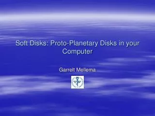
Soft Disks: Proto-Planetary Disks in your Computer Garrelt Mellema
Numerical Models • Reasons to use numerical models: • Reproduce observations / fitting parameters • Observations = radiation, so always requires radiative transfer of some sort. • ‘Experimental’ astronomy: understanding the physics of complex systems: • Disk structure • Planet-disk interaction • Jet collimation • Complex systems: • Gas (atoms, ions, molecules, electrons) / chemistry • Dust (different sizes) • Magnetic Fields • Photons • Gravity (star, binary systems, planets) • In principle we know how to calculate all of these!
Limitations of Numerical Models • In practice one is limited by computational resources. To make calculations feasible one can resort to several simplifications: • Neglect parts of the physics. Can be done if their effects can be included in a simplified way, for example • No magnetic fields, but assume a viscosity for the gas • No dust, but assume it is coupled perfectly to the gas • No radiation, assume that the gas is locally isothermal • Reduce to less than 3 dimensions, for example • Work with surface density for thin disks (h << r) • Assume cylindrical symmetry when studying vertical structure • For continuum processes, one also has to use an (unphysical) discretization (mesh or grid). This implies a finite dynamic range D: L/Δx. Typically D ~100-1000.
Impact of Limitations • As in the case of telescopes, one has to live with the limitations of the tools. • Looking back one can see in the (short) history of computational studies that • Often, adding more details, adds more details in the results (comparison to observations!), but does not change the basic results. • But, in other cases, the added details change the basic results. • Increasing the dimensionality often makes a large difference, especially when it comes to instabilities.
Numerical Gas Dynamics • The equations of gas dynamics are difficult to solve: • Five quantities (8 for magnetohydrodynamics) to solve for. • Non-linear coupled differential equations. • Allow discontinuous solutions (shocks, contact discontinuities). • Two basic approaches are used in astrophysics • Grid-based codes • Quantities defined on a mesh, nowadays often on an adaptive mesh. • Good at discontinuities. • Limitations on spatial dynamic range: bad at following gravitational collapse. • Particle based codes (SPH, Smooth Particle Hydrodynamics) • Quantities associated with particles (representing fluid elements). • Limitations on mass dynamic range. • Good at gravitational collapse. • Bad at discontinuities.
Proto-Planetary Disk Models • Gasdynamic simulations are used to study various processes in proto-planetary disks: • Jet collimation • Planet formation • Turbulence • Disk-Planet interaction
Producing Jets • The collimation of jets & outflows is a classic astrophysical problem, and has been addressed with numerical simulations. • Typically, these simulations the inner disk regions, and the disk is more of a ‘boundary condition’. • Simulations have been showing collimation for decades, however there were always doubts as to the stability of these flows, the flow evolution far away, etc. • There now appears to be a consensus that the jets are magneto-centrifugally launched from a disk-wind, but many open issues remain…
Jets 3D models by Kigure & Shibata (2005). (note: only run for 2 inner-disk orbital perdiods)
Planet Formation • Two models for the formation of massive planets • Core accretion model: slowish growth of planet from first planetesimals, then gas. • Core collapse model: gravitational collapse of parts of a heavy disk. • Both have been studied numerically, with mixed successes. • Core accretion: • Complex physics: sticking planetesimals, coupling to disk dynamics, accretion of gas (on solid). First models: too slow (tformation > 107 years). Nowadays: problem solved…? (opacity, other changes). • Core collapse: • Scale problem, coupled to different physical regimes.
Core Collapse Simulation • SPH Simulation (3D) • Problems: 1) Isothermal equation of state not valid after collapse. 2) Long term stability of the fragments. 3) Role of shocks Attempts to do this problem with grid-based codes have mostly revealed problems with resolving gravitational collapse. Mayer et al. 2002
Magneto-Rotational Instability • Ionized disks are subject to the magneto-rotational instability (MRI), even if only slightly ionized. • Simulations are the only way to evaluate whether MRI can explain the disk ‘viscosity’ needed for accretion. • Results are successful (α ~ few times 10-3), but note that many simulations • Are 2D or 2.5D • Lack dynamic range
Disk-Planet Interaction • A planet embedded in a proto-planetary disk will interact with it. The effects are • Gap opening (affecting accretion to the planet) • Migration (due to angular momentum transfer with the disk) • This problem has been studied extensively with simulations. Most of the results are in 2D and for isothermal disks, often in in co-rotating coordinates. • 2D simulations can be used if the Roche lobe of the planet is either much smaller than the disk scale height (low mass planets), or much larger (high mass planets). • Low mass planets do not open gaps (type I migration). • High mass planets open gaps (type II migration).
Disk-Planet Interaction: 2D/3D • Migration time against planet mass (in stellar masses). • The lines indicate the analytical estimates for Type I and II migration. • 2D: ◊ 3D: ● • The models follow mostly the expected type I and type II migration. • The big difference occurs around the transition between the two: Roche lobe of planet is approaching scale height of disk. Type I Migration time Type II
Planet-Disk Code Comparison • Within the framework of the RTN Formation of Planetary Systems, a comparison of the results for a large range of codes was made. • Four standard problems (Jupiter/Neptune, inviscid/ viscosity) in 2D. • Seventeen codes. • One of the first detailed code comparisons for a complex astrophysical problem. • Detailed results can be found at http://www.astro.su.se/groups/planets/comparison/
Code Overview • Upwind methods • NIRVANA-GDA (Gennaro D'Angelo) • NIRVANA-GD (Gerben Dirksen) • NIRVANA-PC (Paul Cresswell) • RH2D (Willy Kley) • GLOBAL (Sebastien Fromang) • FARGO (Frédéric Masset) • GENESIS (Arnaud Pierens) • TRAMP van Leer (Hubert Klahr) • High-order finite-difference methods • Pencil (Wladimir Lyra) • Shock-capturing methods • AMRA (Pawel Ciecielag & Tomasz Plewa) • Flash-AG (Artur Gawryszczak) • Flash-AP (Adam Peplinski) • TRAMP-PPM (Hubert Klahr) • Rodeo (Sijme-Jan Paardekoper & Garrelt Mellema) • JUPITER (Frédéric Masset) • SPH methods • SPHTREE (Ken Rice) • ParaSPH (Christoph Schäfer & Roland Speith)
Code Comparison Results Invisid Jupiter case
Code Comparison Results (2) Invisid Jupiter case
Code Comparison Results (3) Invisid Jupiter case
Comparison: Density Profiles L4 L5 Density profile along the planet’s orbit Density profile perpendicular to planet’s orbit
Code Comparison Conclusions • PPM codes in co-rotating coordinates show ‘ripples’. • FLASH in cartesian coordinates does not reproduce the gap structure well. • SPH codes do not reproduce the gap structure well. • Other codes (upwind & shock-capturing) roughly agree on gap structure. • But: torques easily different by 50%!
Dust-Gas Coupling • Proto-planetary disks consist of dust and gas. • Gas orbits at slightly sub-Keplerian velocities due to pressure gradient. • Dust wants to orbit at Keplerian velocity (no pressure), but feels the drag of the gas. • Small dust particles (1-10μm) couple well to the gas. • Larger dust particles experience dust drift: gas-dust separation. Especially strong near gradients in gas pressure. • Dust is observationally important: most of the emitted radiation comes from dust. • Rule of thumb: λ ~ dust size.
Dust Emission from Gas Disk Model Wolf et al. 2002 Jupiter-mass planet at 5.2 AU Image at 0.7 mm 4 hour integration with ALMA Assumes perfect dust-gas coupling!
Gas-Dust Disk Model • Planet: 0.1 MJ (no gap in gas!) • Dust:1.0 mm Paardekooper & Mellema (2004)
Dust Emission at λ=1 mm Gas and dust perfectly coupled 0.1 MJup at 5.2 AU, d=140pc, 12mas resolution (ALMA-like) With dust drift