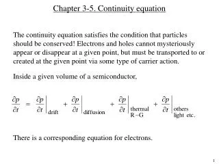
The Continuity Equation
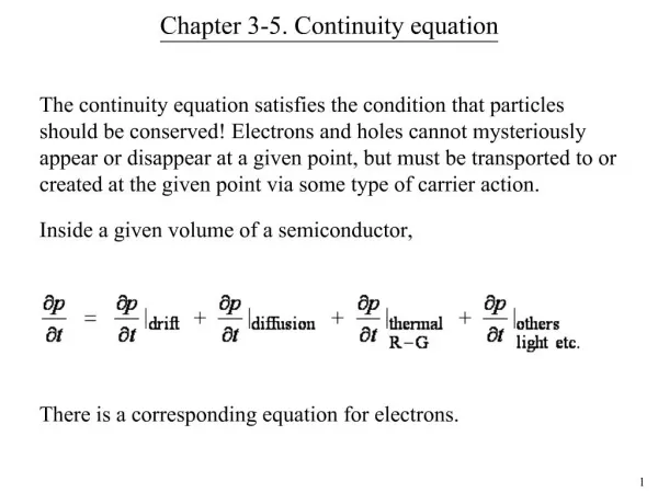
The Continuity Equation. This equation is pervasive, appearing in many different aspects of science and engineering. We ’ ll investigate its form and usage for water flow across a floodplain. Q in. Q out. Cross Section of a Floodplain. t 3. Terre-Firme. t 2. t 1. Floodplain.

The Continuity Equation
E N D
Presentation Transcript
The Continuity Equation This equation is pervasive, appearing in many different aspects of science and engineering. We’ll investigate its form and usage for water flow across a floodplain.
Qin Qout Cross Section of a Floodplain t3 Terre-Firme t2 t1 Floodplain River Channel Q is Discharge t is time
A “Glass” of Water Glass is empty at t1
Qin Qout A “Glass” of Water Qout < Qin t2 ΔS increases Glass is filling at time t2
Qin Qout A “Glass” of Water Qout < Qin t3 ΔS increases t2 Glass is nearly full at t3
Qin Qout A “Glass” of Water Qout > Qin t3 ΔS decreases t4 Glass is emptying at t4
Qin Qout The Basic Form of the Continuity Equation ΔS = Qin - Qout t1 t2 t3 t4 Qout<Qin Qout<Qin Qout>Qin The water flowing into the glass (Qin) minus the water flowing out of the glass (Qout) equals the amount of water that was added to or taken away from the glass (ΔS) during the time step (e.g., t2 to t3). For example, say a sink faucet is filling your glass at 2 gal/min and you have a straw sucking out 0.5 gal/min. And, you do this for one minute. Then the glass will gain 1.5 gallons of water.
What is “Discharge” • Q is discharge, which we typically think-of as the flow of water down a river. • This flow, or Q, is estimated by measuring the river cross-section and measuring the velocity of the water, then multiplying these together.
River Discharge Q = 3m * 10 m * 1 m/s = 30 m3/s Q = 9m * 10 m * 2 m/s = 180 m3/s
How to Apply Continuity to a Floodplain • Why is it difficult to know Q on a floodplain? We can estimate Q in a river channel, but measuring flow velocities on a floodplain or measuring cross sectional area is very difficult (without satellites). • Instead, need to describe the continuity equation with things that are measurable, so… what is easily measured? • the water surface elevation, call that “h” • h on a number of different days, or every hour, or every week, etc., call that “Δh/Δt”, the change in h with the change in time • h at a number of different locations across the floodplain, call that “Δh/Δx”, the change in h with space, ie, the slope
The Amazon Floodplain Its difficult to know the flow velocities and depths in these environments. Characterizing the entire location would take too many surveys. This situation is unlike a typical river channel. However, it should be straightforward to measure the water surface elevation, h.
A “Cube” of Water Qin Qout Qin Qout Qout Imagine the floodplain to consist of a entire series of small cubes of water. Our goal is to describe the flows into and out-of each cube using h as the primary, measurable item. Then, summing each cube will give the Q for the floodplain.
A “Cube” of Water Vin along z axis ΔY ΔZ Vout along y axis Vin along y axis X1 ΔX ΔX = X1 – X2 X2 Vout along z axis Because Q = velocity * area we can use Vin VoutΔX, ΔY, and ΔZ instead of Q Note: V along Y axis is part of this schematic, but not shown for clarity of the drawing.
ΔY ΔY = ΔQy Some Algebra Vin(y) – Vout(y) = ΔVy this is the difference in velocity flowing into and out of the cube along the y axis, or you can think of it as the change in velocity that occurs inside the cube. ΔVy * ΔX * ΔZ = ΔQy Multiplying the change in velocity by the cross sectional area of the cube gives the change in discharge that occurs inside the cube along the y axis. ΔVy * ΔX * ΔZ * Here, multiplying ΔY/ΔY is the same as multiplying by 1, but ΔX * ΔY * ΔZ is the volume of the cube, lets call the volume, “vol” ΔVy * Using this same approach, there are similar expressions for the change in discharge within the cube for the X and Z axis. ΔVx * ΔVz * vol ΔY = ΔQy vol ΔX vol ΔZ = ΔQx = ΔQz
A Little More Algebra Qin – Qout = ΔQ This is an expression that says that all of the flow into the cube minus all of the flow out of the cube is equal to the flow change that occurs inside the cube. ΔQ = ΔQx + ΔQy + ΔQz The total flow change the occurs inside the cube is equal to the sum of the three parts. ΔQ = ΔVx + ΔVy + ΔVz vol ΔX vol ΔY vol ΔZ These are a series of simple algebraic steps replacing variables with their equivalent expressions. ΔVx ΔX ΔVy ΔY ΔVz ΔZ ΔQ = vol ( + + ) ΔVx ΔX ΔVy ΔY ΔVz ΔZ ΔS = vol ( + + ) This is the basic form of the continuity equation. We want this equation in terms of h, the thing we can easily measure.
ΔVx ΔX ΔVy ΔY ΔVz ΔZ ΔS = vol ( + + ) A Basic Physics Fact for Water • Water flows downhill! • An expression for this is: • Applying this expression to the algebra: • What is Δ(Δh)? • How do we re-write ΔS as something with h, the thing that is measurable? Velocity = Constant * Slope Δh ΔX Δh ΔY Δh ΔZ Vx = K * Vy = K * Vz = K * K * Δ(Δh) ΔX * ΔX K * Δ(Δh) ΔY * ΔY K * Δ(Δh) ΔZ * ΔZ ΔS = vol ( + + )
The Continuity Equation for a Floodplain • Δ(Δh)/(ΔxΔx) is the change in water slope. • Recall that ΔS is a measure of the time of Qin and Qout. In the algebra of the cube (i.e., the glass), the glass doesn’t change its size with time, only the water level in the glass changes. So ΔS during the time interval is Δh/Δt. Δ(Δh) ΔX * ΔX Δ(Δh) ΔY * ΔY Δ(Δh) ΔZ * ΔZ Δh/Δt = vol*K ( + + )
Applying the Continuity Equation to a Floodplain • All of the proceeding was to determine K, it is unknown. • To determine K, we’ll use the continuity equation from a number of locations and times. • We’ll simplify the equation to just the x dimension. Δ(Δh) ΔX * ΔX Δh/Δt = h*K ()
Applying the Continuity Equation to a Floodplain Terre-Firme t1 t2 Floodplain River Channel Q is Discharge t is time Here’s the floodplain water level at two different times. The simple form of the continuity equation needs h and x. What are these in this schematic?
Applying the Continuity Equation to a Floodplain h t1 t2 x This is h at two different times for all of the x values. To solve the continuity equation, we need Δ(Δh)/(ΔxΔx) which is the change in slope. Next slides give the slope and then the change in slope.
Applying the Continuity Equation to a Floodplain h These are the rise, or Δh, it’s the difference in h values. Lines have different Δh values, thus different slopes. Note that Δh is negative. t1 This is the run, or Δx, it’s the difference in x values. Both lines have the same Δx. t2 x Slope is rise over run. The t1 line has a shallow slope compared to the t2 line, which has a steeper slope.
Applying the Continuity Equation to a Floodplain x t1 Δh/Δx t2 Because line t2 has a steeper slope than line t1 and because both slopes are negative, line t2 plots below line t1. Now, what is the change in slope?
Applying the Continuity Equation to a Floodplain x This is the change in x, the run. Δh/Δx These are the change in slope. Note that the change in slope is negative. t1 t2 Change in slope is found the same way as finding slope, using the rise over run method.
Applying the Continuity Equation to a Floodplain x Δ(Δh)/(ΔxΔx) t1 t2 Because line t2 has a steeper change in slope than line t1 and because both change in slopes are negative, line t2 plots below line t1.
Applying the Continuity Equation to a Floodplain • Now, we’ve got all of the values for the right hand side of the equation (except K, which we’ll solve for). • What is the left hand side of the equation? Δ(Δh) ΔX * ΔX Δh/Δt = h*K ()
Applying the Continuity Equation to a Floodplain h t1 t2 x This is h at two different times for all of the x values. So Δh is the difference in h values for the two times.
Applying the Continuity Equation to a Floodplain Δh x This is Δh calculated from times t1 and t2.
Applying the Continuity Equation to a Floodplain Δ(Δh) ΔX * ΔX Δh/Δt = h*K () • To determine K, input h, Δh/Δt, and Δ(Δh)/(ΔxΔx) from a given x location. • With K, we can determine velocity anywhere on the floodplain. Recall that: t1 h t2 x Δh x x Δh ΔX Vx = K * t1 Δ(Δh)/(ΔxΔx) t2
Applying the Continuity Equation to a Floodplain • With velocity determined anywhere on the floodplain, we can determine discharge anywhere on the floodplain. • Essentially, discharge in a river channel requires just one cross-section because water is confined to flow between the banks of a river. • Water on a floodplain can move in many different directions. It is not confined by the banks of the river. • Discharge on the floodplain requires knowledge of all “cross-sections” where flow might go. So, if we know the floodplain topography and the h surface, we can calculate the “cross-sections”, these are just the difference between h and topography. • The next slide presentation shows the two-dimensional version of this equation.