Download
1 / 22
220 likes | 385 Views
Compression of Digital Elevation Maps using Nonlinear Wavelets. Prof. Charles D. Creusere Klipsch School of Electrical & Computer Engineering New Mexico State University. Email: ccreuser@nmsu.edu. Topics. Introduction Max- and Min-Lifted Wavelets Qualitative Analysis

E N D
Compression of Digital Elevation Maps using Nonlinear Wavelets Prof. Charles D. Creusere Klipsch School of Electrical & Computer Engineering New Mexico State University Email: ccreuser@nmsu.edu
Topics • Introduction • Max- and Min-Lifted Wavelets • Qualitative Analysis • Compression Comparisons • Conclusions
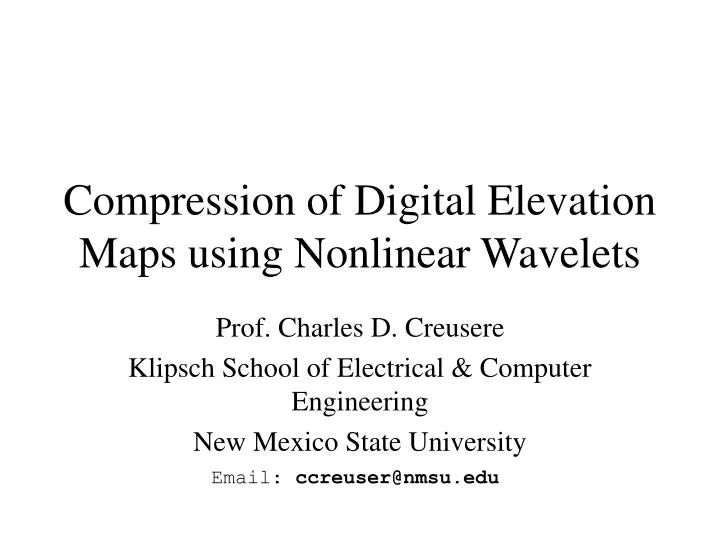
Compressed Database Mobile Field User Hardwired User Introduction Operating Paradigms for DEM Client-Server Interactions Mobile Field User Regional Information Center Stationary Field User
Introduction • Conventionally, digital elevation map (DEM) data is stored simply as a 2-dimensional array which has been referenced to some area on the surface of the earth • Advantages: • Facilitates easy access to every elevation post • No information is lost • Disadvantages: • Requires a lot of memory or communications bandwidth to store or transmit • Data is not well organized for contextual search
Introduction • Our goal is to develop a new digital representation for DEM data that: • Preserves all of the information (i.e, is lossless) • Requires fewer bits to represent the information (i.e., is compressed) • Facilitates efficient search and retrieval (i.e., a minimal number of bits are transmitted/decoded to extract the required information)
Introduction • Our approach: • Transform the DEM data using non-linear max- or min-lifted wavelets • These preserve maxima or minima in the data over local regions • Encode the resulting coefficients from coarse to fine with regionally localized dependencies • i.e., only those coefficients corresponding to the same region in the DEM should have dependencies
2 2 p(s)(n) p(s)(n) l(v)(n) l(v)(n) + + + + 2 2 z z -1 -1 Max- and Min-Lifted Wavelets Analysis Synthesis s(n) = x(2n) s’(n) x(n) + + + - - v’(n) + y(n) + + v(n) = x(2n-1) Predictor: p(s)(n) = max/min(s(n), s(n+1)) Update: l(s)(n) = max/min(0, s(n), s(n+1)) v’(n) = v(n) - max/min(s(n), s(n+1)) => s’(n) = s(n) - max/min(v’(n), v’(n+1))
Max- and Min-Lifted Wavelets Abstract View: coarse input fine details Multiresolution: coarse input details finest details
Max- and Min-Lifted Wavelets • Why? • Low complexity • In-place calculation => memory efficient • No data expansion in transform domain • No initial compression penalty • Unique capability: Maximal (or minimal) values within a 5-point neighborhood are preserved • Facilitates multiresolutional searches for low or high points in DEM data
Max- and Min-Lifted Wavelets • Difficulty: • The exact correspondence between the local minima or maxima at different scales is not entirely deterministic • The output can appear in one of 2 positions • This could make the encoding process more difficult • i.e., it affects the allowable coding dependencies
Qualitative Analysis: Max-Lifting Example: Maxima Localization #1 #4 #6 Input = (1,1,1,1,1,5,1,1) Coarse = (1,1,5,5) Input = (5,1,1,1,1,1,1,1) Coarse = (5,1,1,1) Input = (1,1,1,5,1,1,1,1) Coarse = (1,5,5,1) #2 #5 #7 Input = (1,5,1,1,1,1,1,1) Coarse = (5,5,1,1) Input = (1,1,1,1,5,1,1,1) Coarse = (1,1,5,1) Input = (1,1,1,1,1,1,5,1) Coarse = (1,1,1,5) #3 #8 Input = (1,1,5,1,1,1,1,1) Coarse = (1,5,1,1) Input = (1,1,1,1,1,1,1,5) Coarse = (1,1,1,5)
Qualitative Analysis: Max-Lifting Example: Minima Localization #1 #4 #6 Input = (1,5,5,5,5,5,5,5) Coarse = (1,5,5,5) Input = (5,5,5,1,5,5,5,5) Coarse = (5,5,5,5) Input = (5,5,5,5,5,1,5,5) Coarse = (5,5,1,5) #2 #7 #5 Input = (5,1,5,5,5,5,5,5) Coarse = (5,5,5,5) Input = (5,5,5,5,5,5,1,5) Coarse = (5,5,5,5) Input = (5,5,5,5,1,5,5,5) Coarse = (5,5,1,5) #3 #8 Input = (5,5,1,5,5,5,5,5) Coarse = (5,1,5,5) Input = (5,5,5,5,5,5,5,1) Coarse = (5,5,5,5)
Coarse/ Coarse Fine/ Coarse …. …. Coarse/ Fine Fine/ Fine …. Coarse Fine 2-D Max-/Min-Lifting • A separable 2-d decomposition is formed by first applying the 1-d filter bank to the rows of the array and then applying it to the columns: i.e., Filter Horizontally Filter Vertically 2D Decomposition
Compression Comparisons • We have thus far considered two coding algorithms: Stack-Run and SPIHT • Both are operated losslessly • Stack-Run: low complexity, coarse-to-fine encoding, exploits only intra-scale (subband) redundancy • SPIHT: Rate embedded, exploits both intra- and inter-scale redundancy
Compression Comparisons Coarse-to-Fine Encoding Inter-Scale Dependency • SPIHT exploits redundancies in small values
Compression Comparisons • Data provided by China Lake: • Swath10, Swath3: tiled for coding • Cosogeo10, Cosogeo3 • Transforms evaluated: • Max-lifted • Min-lifted • (2,2)-integer • LZ77 (gzip)
Compression Comparisons • Average Results: Lossless SPIHT • Max-lifted: • 10 meter: 2.539 bits/post, 37202 significant coefficients • 3 meter: 1.366 b/p, 275095 significant coefficients • Min-lifted: • 10 meter: 2.553 b/p, 37184 significant coefficients • 3 meter: 1.374 b/p, 290814 significant coefficients • (2,2)-integer: • 10 meter: 1.879 b/p, 22960 significant coefficients • 3 meter: 1.233 b/p, 183397 significant coefficients
Compression Comparisons • Average Results: Lossless Stack-Run Coding • Max-lifted: • 10 meter: 3.201 bits/post, 37202 significant coefficients • 3 meter: 1.840 b/p, 275095 significant coefficients • Min-lifted: • 10 meter: 3.213 b/p, 37184 significant coefficients • 3 meter: 1.846 b/p, 290814 significant coefficients • (2,2)-integer: • 10 meter: 2.066 b/p, 22960 significant coefficients • 3 meter: 1.318 b/p, 183397 significant coefficients
Compression Comparisons • LZ77 (gzip) Baseline: • 10 meter: 6.264 bits/post (CR = 2.5:1) • 3 meter: 2.633 bits/post (CR = 6:1) • Worse performance than any of the transform-based algorithms because it doesn’t take the specific structure of the data into account
Conclusions • Raw compression efficiency is reduced by using max-/min-lifted wavelets • Exploiting inter-scale redundancy is more important for max-/min-lifted wavelets than for (2,2)-integer wavelet • The results are promising: a 10% increase in file size in exchange for the ability to precisely preserve regional altitude extremes at coarse scales (3 meter data)
Future Research • Quantify the correlations between coefficient at different scales • Using these statistics to optimize a non-embedded, coarse-to-fine coding algorithm for DEM data • Alter this optimized algorithm so that spatial regions can be independently decoded