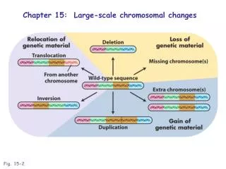
Fig. 2:
Examining Buoyancy Waves in the Martian Atmosphere with Mars Climate Sounder Robert M. Edmonds, J.R. Murphy, D.A. Teal New Mexico State University, Department of Astronomy. Introduction. Analysis Cont. MCS Results.
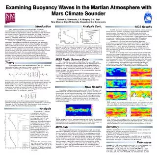

Fig. 2:
E N D
Presentation Transcript
Examining Buoyancy Waves in the Martian Atmosphere with Mars Climate Sounder Robert M. Edmonds, J.R. Murphy, D.A. Teal New Mexico State University, Department of Astronomy Introduction Analysis Cont. MCS Results Many physical processes can create waves in the Martian atmosphere’s thermodynamic and kinetic state. Waves can develop in response to time-varying insolation, referred to as thermal tides. Waves can also develop because of airflow over topography, wind shear instabilities, convection, etc. Many of these waves can have characteristics as those of gravity (i.e. buoyancy) waves due to air parcels being displaced into surrounding air of differing density. Creasey et al. (2006) investigated the amplitudes of Martian atmospheric gravity waves by attempting to determine their manifested temperature perturbations as derived from Mars Global Surveyor (MGS) radio occultation measurements. Their results showed little correlation between topographic variance and gravitational wave energy. Motivated by this result, we are interested in how wave energies derived from Mars Climate Sounder (MCS) limb radiance measurements compare to the MGS Radio Science (RS) results. The low vertical resolution of the MCS measurements likely limit us to investigation of long wavelength gravity waves and thermal tides, but offers the opportunity to systematically investigate wave characteristics diurnally, seasonally, and geographically, and to do so to a higher altitude (lower pressure) than the MGS RS profiles afforded. For MCS Ep analysis limited to 10-40 km above the surface, a vertical domain similar to the MGS RS analysis, results differ from the MGS RS results (compare Fig. 4a with Fig. 3). The MCS results don’t exhibit increased longitudinally continuous equatorial amplitude maxima, but do exhibit enhanced activity in the Tharsis region. These differences are maybe not surprising since the higher vertical resolution MGS RS data likely contributes to a higher sensitivity to the full gravity wave spectrum. If the waves in Fig. 4a are vertically propagating, we expect amplitudes of the perturbations to increase with height. We conducted an analysis at higher altitudes with the same vertical extent of 30 km. Wave amplitudes in the Tharsis region do increase with increasing height as apparent when comparing Fig. 4a 4b 4c & 4d. There are also regions of wave activity that do not seem to propagate vertically, such as the northern subtropics near 120o E. Since the 30 km vertical extent of our analysis window constrains the maximum vertical wavelengths explored in our analysis, we removed that constraint byapplying our analysis to the full vertical extent available in the MCS data. This analysis exhibited prominent equatorial maxima (Figure 5a), which is comparable to the MGS RS results. Note, however that these peak MCS amplitudes are a factor ~8 greater than the MGS RS results & a factor of ~3 greater than the MCS results with the 30 km vertical window. To isolate shorter wavelengths a high -pass filter was applied to the T’(z) profiles, resulting in similar Ep amplitudes as the 30 km window results. Fig. 2: Several synthetic temperature profiles were created and processed to see how the analysis performed. In the left plot, Profile #2 is a median of 214 MCS temperature profiles from Ls 90-135, Latitude 20o-35o, Longitude 0o-15o, & LTST 0200-0600, to which wave perturbations have been added. Profile #1 is the best 3rd order polynomial fit to the unperturbed Profile #2. The wave perturbations consist of long (λ=30 km) and short (λ=10 km) wavelength oscillations with the amplitude exponentially increasing with height. In the plot to the right we see the retrieved short wavelength temperature perturbations from each profile via the analysis and application of the highpass filter. MGS Radio Science Data Theory We first applied our analysis to Mars Global Surveyor (MGS) radio occultation data. The analysis of these data provide an important test of our application of Creasey et al.’s (2006) methods. The complete MGS radio occultation data set provides 21,243 temperature profiles, covering much of the Martian surface and typically extending from the surface to ~45 km in altitude. [Creasey et al. (2006) had only 13,141 profiles available when they conducted their investigation.] For this analysis we interpolated MGS RS temperature profiles to a fixed vertical grid with a spacing of 1.25km, only using profiles between 0200 - 0600 LTST with continuous coverage from 10-30 km in altitude. This was in an attempt to reproduce the methodology of Creasey et al. (2006). The reduction method used in retrieving temperature profiles from MGS RS data is described by Hinson et al. (1999). To investigate waves in the Martian atmosphere (see Fig. 1) we probe the gravitational wave energy per unit mass in our analysis. Total gravitational wave energy per unit mass, E0, is given by, where u' and v’ are the orthogonal horizontal components of the perturbed wind velocity, w' is the vertical component of the perturbed wind velocity, N is the Brunt-Väisälä frequency, g is the acceleration due to gravity (for the Martian surface 3.741 m/s), T0 is the background temperature, T' is the temperature perturbation created by the wave, Ek is the kinetic wave energy per unit mass, and Ep is the potential wave energy per unit mass. The measurable quantity for our data is Ep given by, MGS Results Overall our analysis produced results similar to those of Creasey et al. (2006). Maximum annually and 10-30 km averaged Ep values occurred at equatorial and northern subtropical latitudes. There is a preference for larger Ep magnitudes in the western hemisphere Tharsis upland longitudes (see Fig. 3). Our analysis does not retrieve some southern hemisphere features apparent in Creasey et al.’s (2006) results. Limiting our analysis to only those profiles available to Creasey et al. (2006), these minor differences could not be resolved. According to linear theory Ek/Ep remains constant, so investigation of the potential wave energy should also be probing the wave kinetic & total energy (Tsunda et al. 2000, Van Zandt 1985). Below we apply the Ep analysis to MGS RS & MRO MCS derived temperature profiles. Fig. 4: The Ep distribution from the MCS data at different altitudes. The vertical domain for each map is listed above. The data were spatially binned in the same manner as in Fig. 3. If no data were available in a spatial region than the map was left blank in that region. Analysis To determine Ep, analysis of temperature profiles is conducted. Each temperature profile (interpolated to a fixed vertical grid) is fit with 3rd order polynomials (see Fig. 1). As determined by previous terrestrial investigations, this fit is usually the most appropriate for T0(z) in the calculation of Ep (Tsunda et al. 2000). The deviations of the temperature profile from this fit are used as T‘(z) values. For some Ep calculations the T’(z) profile was low- or high-pass filtered to isolate long or short vertical wavelength features. Fig. 5: The Ep distribution when investigating most of the vertical extent available from the MCS profiles. The data were spatially binned in the same manner as in Fig. 3. A high-pass filter was applied to the T’(z) profiles before producing the plot on the right. The high-pass filter had a cutoff wavelength of 25 km. Note the amplitude scaling difference in the two plots. Fig. 3: Annually averaged 10-30 km Ep magnitudes determined using all MGS RS temperature profiles available. The map provides values (i.e. a pixel) every 5o by 5o, with each value representing the average Ep for profiles located within 15o by 15o area. The Ep values from each profile are vertically averaged before being averaged with other profiles Summary MCS Data • The MCS results using 10-70 km vertical extent show wave activity in the Martian tropics, biased to the southern hemisphere. • The MCS results using the 10-30 km vertical extent do not exhibit a similar Ep distribution as the MGS RS results. • Because of the lower vertical resolution in the MCS data vs. the MGS RS data, we have yet to disentangle the driving mechanism (i.e. gravity waves, thermal tides) behind the Ep distribution in the MCS results. MCS is an infrared radiometer that acquires limb, nadir and off-nadir observations (McCleese et al. 2007). The temperature data used here were derived as outlined by Kleinböhl et al. (2009). Our analysis was conducted on 1,266,250 MCS profiles. While the profiles do not extend to the surface, they typically extend from ~10 - 85 km in altitude. This allows us to explore a vertical domain not achieved by the MGS RS data. The MCS data typically provide ~4 km vertical resolution in the profiles. For our analysis, the profiles were interpolated to a grid with a spacing of 2 km and only those profiles providing continuous vertical coverage in the domain of interest and errors less than 25 K (MCS data provides temperature error information) were included. As with the MGS RS analysis, only profiles with an LTST of 0200 to 0600 were used. Fig. 1: Interpolated MCS temperature profiles (dots in left panels) and their best fit 3rd order polynomials (solid line in left panels). In the panels to the right are the resulting Ep values for the profiles, with the top panel exhibiting much more wave energy. References Creasey, J.E., et al., 2006, Geophys. Res. Lett., 33, L01803; Hinson, D.P., Simson, R.A., Twicken, J.D. & Tyler, G.L. 1999, 104, E11, 26997; Kleinböhl, A.K. et al. 2009, JGR, 114, E10006; McCleese, D.J., et al. 2007, JGR, 112, E05S06; Tsunda, T., Nishida, N., Rocken, C. & Ware, R.H. 2000, JGR, 105, 7257; Van Zandt, T.E. 1985, Radio Sci. 20, 1323