Computational problems, algorithms, runtime, hardness
Computational problems, algorithms, runtime, hardness (a brief introduction to theoretical computer science) slides by Vincent Conitzer. Set Cover (a computational problem ). We are given: A finite set S = {1, …, n} A collection of subsets of S: S 1 , S 2 , …, S m We are asked:

Computational problems, algorithms, runtime, hardness
E N D
Presentation Transcript
Computational problems, algorithms, runtime, hardness (a brief introduction to theoretical computer science) slides by Vincent Conitzer
Set Cover (a computational problem) • We are given: • A finite set S = {1, …, n} • A collection of subsets of S: S1, S2, …, Sm • We are asked: • Find a subset T of {1, …, m} such that Uj in TSj= S • Minimize |T| • Decision variant of the problem: • we are additionally given a target size k, and • asked whether a T of size at most k will suffice
Set Cover (a computational problem) • One instance of the set cover problem: • S = {1,2,3,4,5,6}, • S1 = {1,2,4}, • S2 = {3,4,5}, • S3 = {1,3,6}, • S4 = {2,3,5}, • S5 = {4,5,6}, • S6 = {1,3} • Can you see why it is hard?
Visualizing Set Cover • S = {1, …, 6}, S1= {1,2,4}, S2= {3,4,5}, S3= {1,3,6}, S4= {2,3,5}, S5= {4,5,6}, S6= {1,3} 2 3 4 1 6 5
Using glpsol to solve set cover instances • How do we model set cover as an integer program? • See examples
Algorithms and runtime • We would see: • the runtime of glpsol on set cover instances increases rapidly as the instances’ sizes increase • if we drop the integrality constraint, can scale to larger instances • Questions: • Using glpsol on our integer program formulation is but one algorithm – maybe other algorithms are faster? • different formulation; different optimization package (e.g., CPLEX); simply going through all the combinations one by one; … • What is “fast enough”? • Do (mixed) integer programs always take more time to solve than linear programs? • Do set cover instances fundamentally take a long time to solve?
A simpler problem: sorting • Given a list of numbers, sort them • (Really) dumb algorithm: Randomly perturb the numbers. See if they happen to be ordered. If not, randomly perturb the whole list again, etc. • Reasonably smart algorithm: Find the smallest number. List it first. Continue on to the next number, etc. • Smart algorithm (MergeSort): • It is easy to merge two lists of numbers, each of which is already sorted, into a single sorted list • So: divide the list into two equal parts, sort each part with some method, then merge the two sorted lists into a single sorted list • … actually, to sort each of the parts, we can again use MergeSort!
Polynomial time • Let |x| be the size of problem instance x • Let a be an algorithm for the problem • Suppose that for any x, runtime(a,x) < cf(|x|) for some constant c and function f • Then we say algorithm a’s runtime is O(f|x|) • a is a polynomial-time algorithm if it is O(f(|x|)) for some polynomial function f • P is the class of all problems that have at least one polynomial-time algorithm • Many people consider an algorithm efficient if and only if it is polynomial-time
Two algorithms for a problem 2n 2n2 runtime run of algorithm 1 run of algorithm 2 Algorithm 1 is O(n2) (a polynomial-time algorithm) Algorithm 2 is not O(nk) for any constant k (not a polynomial-time algorithm) The problem is in P
Linear programming and (mixed) integer programming • LP and (M)IP are also computational problems • LP is in P • Ironically, the most commonly used LP algorithms are not polynomial-time as an upper bound (but “usually” polynomial time) • (M)IP is not known to be in P • Most people consider being in P unlikely
Reductions • Sometimes you can reformulate problem A in terms of problem B so that solving B solves A (i.e., reduce A to B) • E.g., we have seen how to formulate several problems as linear programs or integer programs • In this case problem A is at most as hard as problem B (B could be harder) • For example, could get a cookie by donating blood, but donating blood is tougher. • Since LP is in P, all problems that we can formulate using LP are in P • Caveat: only true if the linear program itself can be created in polynomial time!
NP (“nondeterministic polynomial time”) • Recall: decision problems require a yes or no answer • NP: the class of all decision problems such that if the answer is yes, there is a simple proof of that • E.g., “does there exist a set cover of size k?” • If yes, then just show which subsets to choose! • Technically: • The proof must have polynomial length • The correctness of the proof must be verifiable in polynomial time
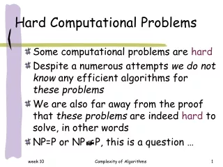
P vs. NP • Open problem: is it true that P=NP? • The most important open problem in theoretical computer science (maybe in mathematics?) • $1,000,000 Clay Mathematics Institute Prize • Most people believe P is not NP • If P were equal to NP… • Current cryptographic techniques can be broken in polynomial time • Computers can probably solve many difficult mathematical problems… • … including the other Clay Mathematics Institute Prizes!
NP-hardness • A problem is NP-hard if the following is true: • Suppose that it is in P • Then P=NP • So, trying to find a polynomial-time algorithm for it is like trying to prove P=NP • Set cover is NP-hard • Typical way to prove problem Q is NP-hard: • Take a known NP-hard problem Q’ • Reduce it to your problem Q • (in polynomial time) • E.g., (M)IP is NP-hard, because we have already reduced set cover to it • (M)IP is more general than set cover, so it can’t be easier • A problem is NP-complete if it is 1) in NP, and 2) NP-hard
Reductions: To show problem Q is easy: reduce Problem known to be easy (e.g., LP) Q To show problem Q is (NP-)hard: reduce Problem known to be (NP-)hard (e.g., set cover, (M)IP) Q ABSOLUTELY NOT A PROOF OF NP-HARDNESS: reduce Q MIP
Independent Set • In the below graph, does there exist a subset of vertices, of size 4, such that there is no edge between members of the subset? • General problem (decision variant): given a graph and a number k, are there k vertices with no edges between them? • NP-complete
Reducing independent set to set cover 2 1 3 , k=4 5 4 6 9 8 7 • In set cover instance (decision variant), • let S = {1,2,3,4,5,6,7,8,9} (set of edges), • for each vertex let there be a subset with the vertex’s adjacent edges: {1,4}, {1,2,5}, {2,3}, {4,6,7}, {3,6,8,9}, {9}, {5,7,8} • target size = #vertices - k = 7 - 4 = 3 • Claim: answer to both instances is the same (why??) • So which of the two problems is harder?
Weighted bipartite matching 3 4 5 2 1 6 1 3 7 • Match each node on the left with one node on the right (can only use each node once) • Minimize total cost (weights on the chosen edges)
Weighted bipartite matching… • minimize cij xij wherecij is edge cost and xij =1 if edge from i to j is chosen • subject to • for every i, Σj xij = 1 • for every j, Σi xij = 1 • for every i, j, xij ≥ 0 • Theorem [Birkhoff-von Neumann]: this linear program always has an optimal solution consisting of just integers • and typical LP solving algorithms will return such a solution • So weighted bipartite matching is in P