Download
1 / 23
230 likes | 360 Views
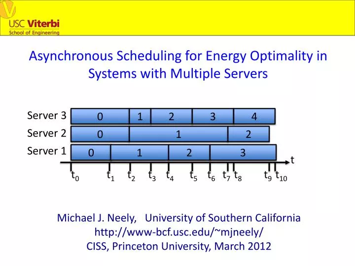
Asynchronous Scheduling for Energy Optimality in Systems with Multiple Servers. Server 3. 0. 1. 2. 3. 4. Server 2. 0. 1. 2. Server 1. 0. 1. 2. 3. t. t 0. t 1. t 2. t 3. t 4. t 5. t 6. t 7. t 8. t 9. t 10. Michael J. Neely, University of Southern California

E N D
Asynchronous Scheduling for Energy Optimality in Systems with Multiple Servers Server 3 0 1 2 3 4 Server 2 0 1 2 Server 1 0 1 2 3 t t0 t1 t2 t3 t4 t5 t6 t7 t8 t9 t10 Michael J. Neely, University of Southern California http://www-bcf.usc.edu/~mjneely/ CISS, Princeton University, March 2012
Motivation • The following things are important: • Multi-core processing architectures. • Distributed data center processing. • Energy-efficiency.
Server 1 λ1 λ2 Server 2 λΝ Server S • N classes of jobs, with Poisson arrivals. • Jobs are queued according to class: Q1(t), …, QN(t). • S heterogeneous servers. Servers can have… • …different classes that are allowed for service. • …different processing mode options. • …different processing times and energy expenditures.
Consider one particular server: Frame 1 Frame 0 Active Active Active Idle Idle t Ds[0] Ds[2] Ds[1] Is[0] Is[1] • Continuous Time operation. • Each server s in {1, …, S} operates over frames. • At frame r in {0, 1, 2, …}, server s decides: • ms[r] = processing mode for frame r. • (chosen in some abstract set of options Ms). • Is[r] = Idle time for frame r (possibly 0). • (chosen in the interval [0, Imax]).
Affect of Decisions on 1 Frame Frame 1 Frame 0 Active Active Active Idle Idle t Ds[0] Ds[2] Ds[1] Is[0] Is[1] • Choosing ms[r], Is[r] determines: • μsn[r] = # jobs of type n that can be served by s • = μsn(ms[r]) (for each n in {1, …, N}) • es[r] = energy expended by server s • = esproc(ms[r]) + psidleIs[r] • Ts[r] = frame duration for server s • = D(ms[r]) + Is[r] ⌃ ⌃ ⌃
Now put all servers together: Server 3 0 1 2 3 4 Server 2 0 1 2 Server 1 0 1 2 3 t t0 t1 t2 t3 t4 t5 t6 t7 t8 t9 t10 • tk = start of kthsub-frame. • S(tk) = {servers that start a frame at time tk}. • What is the “state” at time tk? • State has size at least 2S. • (because each server is either ACTIVE or IDLE)
A “Simpler” Approach • Look at the time averages that the network can achieve, • and that are necessary. • Define ēs, Ts, μsnas frame averages: • The time average energy for server s is then:
The Optimization Problem • Goal: Minimize total time average power subject to supporting all data (i.e., stabilizing all queues). • Minimum power is given by the following problem: Is this really “simpler”? How to solve this?
Special Case for Intuition • Suppose set of mode options Msis finite for all s. • Can show optimality of stationary, randomized policies • with Is fixed, and with Pr[ms[r] = ms] = qs(ms):
Special Case for Intuition • Suppose set of mode options Msis finite for all s. • Can show optimality of stationary, randomized policies • with Is fixed, and with Pr[ms[r] = ms] = qs(ms):
Reminiscent of a “Linear Fractional (LF) Program” • LF Problems are non-convex, but can be solved efficiently: • Boyd, Vandenberghe book (non-linear change of variables). • Neely 2011 presents online method (for 1-server problem). • Our problem is not LF. It has: • Fractional terms in the constraints. • Fractional terms with different denominators. • Such problems are generally intractable.
Reminiscent of a “Linear Fractional (LF) Program” • LF Problems are non-convex, but can be solved efficiently: • Boyd, Vandenberghe book (non-linear change of variables). • Neely 2011 presents online method (for 1-server problem). • Our problem is not LF. It has: • Fractional terms in the constraints. • Fractional terms with different denominators. • Such problems are generally intractable. • BUT: Our problem has special physical structure!
Main Result • We exploit the physical structure to solve the problem. • Our solution is an online algorithm and: • Does not require knowledge of arrival rates. • Works even if the option sets Ms are infinite. • Adaptive when rates change. • Extends Lyapunov optimization theory to treat coupled systems that operate asynchronously over their own timelines.
We use 2 Ideas from Restless Bandit Theory • Drift-Plus-Penalty Ratio from our prior work • [Li, Neely 2010, 2011]. • View discrete rewards as being continuously integrated over time (similar to Tsitsiklis 94 • “short proof” of Gitten’s index theorem).
Continuously Integrating the Energy Penalty Accumulated energy expenditure for one server s time • Define: Rs(t) = Current frame number of server s. • Define: ps(t) = es[Rs(t)]/Ts[Rs(t)] = penalty rate function. • If t = start of new frame for server s, then:
Continuously Integrating the Energy Penalty Accumulated energy expenditure for one server s time • Define: Rs(t) = Current frame number of server s. • Define: ps(t) = es[Rs(t)]/Ts[Rs(t)] = penalty rate function. • If t = start of new frame for server s, then:
A look at one sub-frame [t4, t5]: Server 3 0 1 2 3 4 Server 2 0 1 2 Server 1 0 1 2 3 t t0 t1 t2 t3 t4 t5 t6 t7 t8 t9 t10 • We have effective penalty rates and effective service rates: • ps(t) = es[Rs(t)]/Ts[Rs(t)] • γsn(t) = μsn[Rs(t)]/Ts[Rs(t)]
A look at one sub-frame [t4, t5]: Server 3 0 1 2 3 4 Server 2 0 1 2 Server 1 0 1 2 3 t t0 t1 t2 t3 t4 t5 t6 t7 t8 t9 t10 • Define Lyapunov function on queue state (Q1(t), …, QN(t)): • L(t) = ∑nQn(t)2 • Define Lyapunov Drift Δ(tk) for sub-frame k: • Δ(tk) = L(tk+1) – L(tk) • Define Drift-Plus-Integrated-Penalty:
Strategy Server 3 0 1 2 3 4 Server 2 0 1 2 Server 1 0 1 2 3 t t0 t1 t2 t3 t4 t5 t6 t7 t8 t9 t10 When it is time for server s to make a decision, it chooses a processing mode and idle time to minimize its contribution to the drift-plus-integrated-penalty expression.
Resulting Algorithm • At each time tk, each server s that starts a new frame at this time does the following: • Observe all queues Q1(tk), …, QN(tk). • Choose mode and idle time decisions msk, Isk to solve: • No knowledge of arrival rates λ1, …, λN. • Decentralized. • Generalizes the max-weight algorithm of Tassiulas& Ephremides1992 to treat multiple asynchronous servers and joint stability and power optimization.
Resulting Algorithm • At each time tk, each server s that starts a new frame at this time does the following: • Observe all queues Q1(tk), …, QN(tk). • Choose mode and idle time decisions msk, Isk to solve: *Note: Given msk, it is easy to show that:
Performance Theorem If the problem is feasible, then: All queues are stable. Average power satisfies for all k in {1, 2, 3, …}: Average queue size is O(V).
Conclusions Server 3 0 1 2 3 4 Server 2 0 1 2 Server 1 0 1 2 3 t t0 t1 t2 t3 t4 t5 t6 t7 t8 t9 t10 • Lyapunov optimization method extended to treat multi-server systems operating over asynchronous timelines. • Non-Convex Fractional Problem is solved. • Algorithm is decentralized at each server. • Algorithm does not require knowledge of • rates (λ1, …, λN).