System Solutions

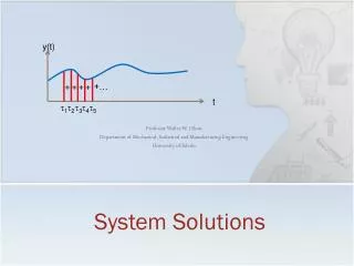
1. System Solutions Professor Walter W. Olson Department of Mechanical, Industrial and Manufacturing Engineering University of Toledo y(t) + + + + +… t t1 t2 t3 t4 t5

2. Outline of Today’s Lecture • Review • Linear Systems • Functions of Square Matrices • Eigenvalues • Stability • Modes • Convolution Equation • Impulse Response • Step Response • Frequency Response • Linearization

3. What is a Linear Systems • In order to be Linear, a system f(x) must obey the rules • So why is this important for controls?

4. Linear Control Systems • If we have two responses known from our system, say, then we also can find the response to the sum of the imput:

5. The Exponential Function of a Square Matrix A • A Taylor series of the exponential function of x is • Thus we can define as the matrix exponential • In Matlab, the comandexpm(A) computes • And we can use this just as we would any other function • For Example, the solution of is and

6. What is a measure of stability? • If you have been paying attention you noted that if the system terms were such thatthe system was stable! • So, can we evaluate in out state space model? If the system is Linear, we can.

7. Eigenvalues • As we are about to find out, the eigenvalues are the key to determining stability • For a square matrix with n rows, the determinant will form an n degree polynomial of the form • Eigenvalues are the roots of this polynominal, that is • Eigenvectors x are the solution to the equation • Many methods exist to find the values of eigenvalues and eigenvetors • In Matlab, the function eig(A) computes the eigenvalues

8. Determination of Stabilityfrom Eigenvalues

9. u Modes x k • Mode: A pattern of motion, sometimes called a mode shape u m x k Mode 1 m Fixed Refe: y Fixed Refe: y Mixed Mode u u Mode 2 x x k k m m m m Fixed Refe: y Fixed Refe: y

10. Modes • Each eigenvalue is associated with a mode of a system • Each eigenvalue is associated with an eigenvector, , such that • If the eigenvalues are distinct, we can form the modal matrix, M, from the eigenvectors and use it to diagonalize the dynamics matrix A which will then separate each mode in the form of a differential equation: • When a set of eignevectors are repeated (equal to each other) a full set of n linear independent eignevectors may or may not exist. In that case we need to form the Jordan blocks for the repeated elements

11. Modes • Jordan blocks have the form • The number of rows and columns of the Jordan block is the number of times (the multiplicity) that the eigenvector is repeated • Then the modes are separated by using the modal matrix as before, but now producing the Jordan form where each block now conforms to a mode.

12. Modes • Modes can be easily found using Matlab function Jordan: • The over decoupling of the system can be represented as >> A A = 1 -3 -2 -1 1 -1 2 4 5 >> [V,D]=eig(A) V = -0.4082 + 0.0000i -0.4082 - 0.0000i -0.7071 -0.4082 - 0.0000i -0.4082 + 0.0000i 0.0000 0.8165 0.8165 0.7071 D = 2.0000 + 0.0000i 0 0 0 2.0000 - 0.0000i 0 0 0 3.0000 >> J=jordan(A) J = 2 1 0 0 2 0 0 0 3

13. Transformations • We can transform our state space representation to other state variables (different that the ones in use). • Mathematically, this is called a change of basis vectors. • Why would we ant to do this? • To make the problem easier to solve! • To isolate a particular property of the system • To uncouple the modes of the system

14. Transformations • Say we have some matrix T that is invertible (this is important) which results in the vector z when x is premultiplied by T. We then say that we have transformed the vector x into z, or alternatively, we have transformed x into z:

15. Solving the Linear System

16. Convolution Equation is called the “Convolution Equation” Expresses the effect of an input on the system • What is convolution? • a twisting or folding together of two things • A convolution is found in many phenomena: • A sound that bounces off of a wall and interacts with the source sound is a convolution • A shadow is a convolution between the light source and the object producing the shadow • In statistics, a moving average is a convolution

17. Convolultion • Example

18. Convolution

19. Convolution

20. Transformations of our solution • A property of matrix exponentials is that • Therefore

21. The Impulse Function • Imagine a function that has a shape that is infinitesimally thin in the independent variable but infinitely high domain or response: • In other words this is a very long and sharp spike • This is what we try to model with the impulse function • Mathematically we define the Dirac Delta Function, d(t), also called the Impulse Function by

22. Properties of the Impulse Function f(t) f(a) t a “Time shift property”

23. System Response Since our system is linear and we can add solutions, we can approximate the response as a sum of the convolutions of h(t-t)d(t) y(t) + + + + +… t t1 t2 t3 t4 t5

24. System Response S(t) • A unit step is defined as • With zero initial conditions 1 { Overshoot Mp t Steady State Rise time, tr Transient period=settling time, ts } } Transient Steady State

25. System Response • Another common test function is a sinusoid for frequency response • Since we have a linear system, we only need and assuming that the eigenvalues A do not equal s } } Steady State Transient

26. System Response: Frequency Response • Time history with respect to a sinusoid: Phase Shift, DT Amplitude Ay Amplitude Au Input Sin(t) Period,T Transient Response

27. System ResponseFrequency Response M is the magnitude and q is the phase

28. Linearization • Good solutions for the Linear Model • Equally good techniques for the Nonlinear Model are not easy to come by • What if the Nonlinear Model is well enough behaved in the region of interest so that we could apply Linear techniques strictly to that region? • We did this with the inverted pendulum! • We assumed small angles!

29. Linearization Techniques • Ignore the nonlinearity • In some cases, the nonlinearity has a relatively small effect • In those cases, build a linear system and treat the nonlinearity as a disturbance • Small angle approximations • Often only useful near equilibrium points • Taylor Series Truncation about an operating point • Assumes that 2nd and higher orders are negligible • Feedback linearization 0

30. Summary S(t) • Convolution Equation • Impulse Response • Step Response • Frequency Response • Linearization 1 t Next: Reachiblity