Groundwater

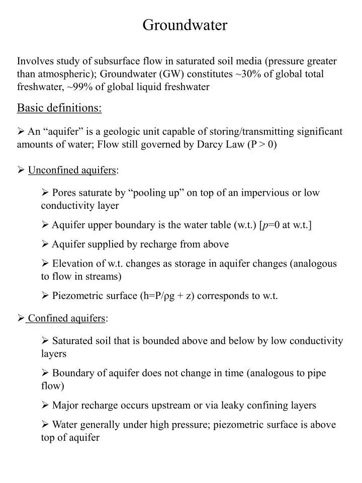
1. Groundwater Involves study of subsurface flow in saturated soil media (pressure greater than atmospheric); Groundwater (GW) constitutes ~30% of global total freshwater, ~99% of global liquid freshwater Basic definitions: • An “aquifer” is a geologic unit capable of storing/transmitting significant amounts of water; Flow still governed by Darcy Law (P > 0) • Unconfined aquifers: • Pores saturate by “pooling up” on top of an impervious or low conductivity layer • Aquifer upper boundary is the water table (w.t.) [p=0 at w.t.] • Aquifer supplied by recharge from above • Elevation of w.t. changes as storage in aquifer changes (analogous to flow in streams) • Piezometric surface (h=P/ρg + z) corresponds to w.t. • Confined aquifers: • Saturated soil that is bounded above and below by low conductivity layers • Boundary of aquifer does not change in time (analogous to pipe flow) • Major recharge occurs upstream or via leaky confining layers • Water generally under high pressure; piezometric surface is above top of aquifer

2. Unconfined vs. Confined Aquifers Figure 6.1.3 (p. 144)Types of aquifers (from U.S. Bureau of Reclamation (1981)).

3. Water Storage in Aquifers Unconfined aquifers: • storage changes correspond directly to change in water table level (w.t. increases = water going into storage and vice versa) storage parameter: “specific yield” or storage coeff. (Sy) = volume of GW released per unit decline in water table (per unit area) Confined aquifers: • storage changes correspond mainly to compression of aquifer as weight of overlying material is transferred from liquid to solid grains (change in porosity) when water is removed (or vice versa) storage parameter: “specific storage” (Ss) Also often use “storativity” (S):

4. Confined aquifer Unconfined aquifer Figure 6.1.5 (p. 145)Illustrative sketches for defining storage coefficient of (a) confined and (b) unconfined aquifers (from Todd (1980)).

5. Derivation of 2D GW Flow Equation From mass balance considerations the 3D GW flow equation is given by: Provided the necessary boundary conditions (2 per spatial dimension) and an initial condition we could solve the above 2nd order PDE for h(x,y,z,t) However, GW flow in aquifers largely consists of horizontal flow (in the x-y plane) Dupuit approx.: We can simplify the equation for these cases by integrating the above equation with respect to z, assuming no vertical flow inside aquifer (qz= 0) and that the aquifer has a horizontal lower boundary (h = h(x,y,t)) We can integrate from z=0 to z=h’, where h’= h (water table) for unconfined aquifers and h’=b (aquifer thickness) for confined aquifers: This equation consists of four terms (one on LHS; three on RHS). We will integrate them one-by-one. First (term #1):

6. Next (term #2): Similarly (term #3), Finally (term #4),

7. Putting the four terms back together to get 2D GW Flow Equations: Confined aquifers: which is a linear PDE; R > 0 only if leaky upper boundary Unconfined aquifers: which is a nonlinear PDE in h. To make the equation linear use: Substituting: Which is linear in the variable h2.

8. By expressing both equations in linear form, we can write a unified governing linear 2D GW flow equation for a homogeneous/isotropic aquifer: where For pumping problems (flow toward a single pumping well) it is useful to write the governing equation in cylindrical coordinates: NOTE: We will often use this equation as the starting point for solving steady-state and/or 1D problems. In the case of steady-1D problems, the above PDE reduces to an Ordinary Differential Equation (ODE) which we can generally easily integrate. The linearity of the governing equation also allows for the application of the principle of superposition.

9. Figure 6.4.4 (p. 159)Well hydraulics for a confined aquifer.

10. Figure 6.4.6 (p. 161)Well hydraulics for an unconfined aquifer.

11. Drawdown for Transient Pumping from a Confined Aquifer Tabulated Well Function Table 6.5.1 (p. 163)Values of W(u) for Various Values of u.

12. Steady-state pumping (single well in infinite confined aquifer)

13. Steady-state pumping (single well in infinite unconfined aquifer)

14. Superposition of GW solutions The linearity of the governing equations in GW flow allow for the application of the principle of superposition of solutions. This means we can “build-up” the solution to a more complicated problem by summing up solutions to simpler problems (that when added together represent the actual GW problem). In the context of pumping wells, we have solutions for a single well in an infinite aquifer; we would like to extend these solutions to more realistic problems. Cases where this idea is useful in pumping problems include: An infinite aquifer with multiple wells Non-infinite aquifers with a no-flux BC Non-infinite aquifers with a fixed-head BC Combinations of the above cases

15. Superposition of Multiple Wells Single well solutions are only strictly applicable for the idealized conditions they were derived under. However linearity of the governing equation allows for superposition of single well solutions. For the case of multiple wells in a confined aquifer, the actual drawdown resulting from all wells can be obtained simply by summing up the drawdown from each single well. Note: Summation of drawdowns not strictly applicable for unconfined aquifers since equations not linear in h (and therefore not linear in drawdown s).

16. Method of Images – No-flux Boundaries s(x,y) = ? In realistic problems we are often dealing with a non-infinite aquifer (i.e. there is some sort of boundary within the radius of influence of the pumping well). In the case above there is an impermeable boundary meaning there is no flux at that boundary. We are interested in solving for the head (or drawdown) profile under these conditions. The differences between the actual head (drawdown) and that predicted by a single pumping well (in an infinite aquifer) solution are: i) The gradient in head must be zero at the boundary, and ii) the presence of the boundary will reduce the flow to the well from that portion of the domain, thereby reducing the head (increasing the drawdown) everywhere as the flow must be replaced from other portions of the domain. We could attempt to solve this more complicated problem numerically, or we can use superposition to our advantage to determine the actual solution.

17. Method of Images – No-flux Boundaries To model the realistic problem, we can use the concept of an “image well” to model the effects of the impermeable boundary. Namely, if we place an image well pumping at the same rate as the real well at a symmetric distance on the other side of the boundary (i.e. as a mirror image) and add up the drawdowns (which we can do due to superposition) we will ensure that: i) The gradient in head is zero at the boundary, and ii) all flow that would have been captured by the real well if it were in an infinite aquifer will instead be captured by the image well, thereby increasing the drawdown everywhere in the real domain. Hence the drawdown anywhere in the domain for the real problem is: Where the drawdown solutions on the right-hand-side are those for an single well in an infinite aquifer. Note: The image well must use a different coordinate since it is as a different location.

18. Method of Images – No-flux Boundaries We can illustrate this with an example. As we’ve seen, for an infinite aquifer with a single well, the drawdown field would look like the following: Symmetric cone of depression

19. Method of Images – No-flux Boundaries If we have a non-infinite aquifer, i.e. with a no-flux boundary, the single well solution obviously no longer holds: Head gradient not equal to zero at boundary However, we can conceptualize the boundary condition as a pumping image well (pumping at the same rate): Image well drawdown (assuming an infinite aquifer) Single well drawdown (assuming an infinite aquifer)

20. Method of Images – No-flux Boundaries If the drawdown from the two single well solutions are summed up, we get the actual resultant drawdown: Note: -- Head gradient is zero at boundary -- Drawdown is increased compared to single well solution.

21. Method of Images – Fixed-head Boundaries The other type of non-infinite aquifer condition we often must deal with is that of a stream boundary. For simplicity, the stream is often modeled as a fixed-head boundary condition. We are interested in solving for the head (or drawdown) profile under these conditions. The differences between the actual head (drawdown) and that predicted by a single pumping well (in an infinite aquifer) solution are: i) The head must equal the fixed-head at the boundary, and ii) the presence of the boundary will increase the flow to the well from that portion of the domain, thereby increasing the head (decreasing the drawdown) everywhere as the flow is augmented by the fixed-head boundary. We could attempt to solve this more complicated problem numerically, or we can again use superposition to our advantage to determine the actual solution.

22. Method of Images – Fixed-head Boundaries To model the realistic problem, we can again use the concept of an “image well” to model the effects of the fixed head boundary. Namely, if we place an image well recharging (negative pumping rate) at the same rate as the real well at a symmetric distance on the other side of the boundary and add up the drawdowns (which we can do due to superposition) we will ensure that: i) The head is equal to the fixed value at the boundary, and ii) all flow that would have been unavailable to the real well if it were in an infinite aquifer (due to drawdown) will instead be supplied by the image well, thereby decreasing the drawdown everywhere in the real domain. Hence the drawdown anyhwere in the domain for the real problem is: Where the drawdown solutions on the right-hand-side are those for an single well in an infinite aquifer. Note: The image well must use a different coordinate since it is as a different location.

23. Method of Images – Fixed-head Boundaries Using the same example as before , but now with a recharge image well, if the drawdown from the two single well solutions are summed up, we get the actual resultant drawdown: Note: -- Drawdown is zero at the boundary -- Drawdown is decreased compared to single well solution.

24. y x Numerical Example • The governing equation for 2D steady-state GW flow in a homogeneous/isotropic confined aquifer (with recharge/ pumping) is: Assume island is square, with a head h=0 meters along the boundary: h=0 h(x,y)=? Spatially varying recharge and non-infinite aquifer make analytical solutions (even with superposition) difficult if not impossible • Need to solve numerically

25. Case 1: • Spatially variable recharge [more recharge away from (x,y) = (0,0)]:

26. Case 2: • Spatially variable recharge with pumping (at 5 wells):

27. In general, 2D/3D GW problems must be solved numerically, i.e. using MODFLOW Figure 6.9.2 (p. 184)Cell map used for the digital computer model of the Edwards (Balcones fault zone) aquifer (after Klemt et al. (1979)). Figure 6.9.4b (cont.)Water levels for Barton Springs—Edwards Aquifer. (b) Perspective block diagram of 1981 water levels viewed from the east side of the aquifer (after Wanakule (1985)).