Understanding Spatially-Structured Evolutionary Algorithms in Computational Intelligence
This document outlines the principles of Spatially-Structured Evolutionary Algorithms (SSEAs) as presented at the Australasian Computational Intelligence Summer School 2009. It introduces fundamental evolutionary algorithm concepts, including mutation, selection, and genetic drift, while emphasizing the importance of spatial structure in evolution. Key topics include island and diffusion models, migration strategies, and the implications of spatial interactions for diversity and evolutionary processes. This content serves as a foundational guide for understanding how spatial structures influence computational intelligence.

Understanding Spatially-Structured Evolutionary Algorithms in Computational Intelligence
E N D
Presentation Transcript
Spatially-Structured Evolutionary Computation Grant Dick Department of Information Science, School of Business, University of Otago, Dunedin, NZ http://www.otago.ac.nz/informationscience/ Australasian Computational Intelligence Summer School, 2009
Overview Basic evolutionary algorithm (EA) model Spatial models of evolution Theory of spatially-structured EAs (SSEAs) SSEA examples and applications Conclusion Australasian Computational Intelligence Summer School, 2009
Basic Terms Individual – candidate solution to problem Population – collection of individuals Deme – subset of population Australasian Computational Intelligence Summer School, 2009
Evolutionary Algorithms (EAs) • Stochastic population-based search methods • “Generate and test” metaphor • Inspired by principles of neo-Darwinian evolution: • Variation (e.g. mutation) • Fitness • Selection (“Survival of the fittest”) Australasian Computational Intelligence Summer School, 2009
Basic EA Model pop = generate and evaluate random population while not done do parents = selection(pop) gen = recombine(parents) evaluate(gen) pop = replacement(pop gen) end while Australasian Computational Intelligence Summer School, 2009
Concepts of Evolution • Mutation • Selection: • Takeover time • Probability of fixation to mutant • Genetic Drift: • “Drunkard’s Walk” • Fixation through chance in a finite population Australasian Computational Intelligence Summer School, 2009
Populations in Space • Populations evolve through time and space: • Spatial structure of populations often ignored • Space divides a population and provides: • Clines (Gradients) • Local competition for resources • Reproductive isolation • Restricted gene flow • Spatial structure important for species development Australasian Computational Intelligence Summer School, 2009
Spatial Models of Speciation Allopatric Parapatric Sympatric Australasian Computational Intelligence Summer School, 2009
Spatial Structure vs. Parallel Exec. • Spatial structure does NOT imply parallel execution: • Parallel execution (e.g. Fitness evaluation) needs no structure (e.g. master-slave model) • However, spatial structure provides logical framework for parallelisation Australasian Computational Intelligence Summer School, 2009
SSEAs • Inspired by models of biological evolution • Limit interactions between individuals through topological constraints • Two main approaches: • Island models • Diffusion models • Basic EA can be thought of as a special case SSEA (called a panmictic EA) Australasian Computational Intelligence Summer School, 2009
Island Model EAs • Multiple population extension to simple EA • Basic operators unchanged: • e.g. selection, recombination, mutation • Introduction of migration operators Australasian Computational Intelligence Summer School, 2009
Island Model EAs Islands Australasian Computational Intelligence Summer School, 2009
Island Model EA pop = generate and evaluate random population while not done do for each island immigrants = select_migrants(pop, topology) insert_immigrants(island, immigrants) next for each island /* perform simple EA iteration within island */ next end while Australasian Computational Intelligence Summer School, 2009
Migration Australasian Computational Intelligence Summer School, 2009
Migration • Exchange of individuals between islands • Promote restoration of intra-island diversity • Parameters: • Topology • Rate (how often, how many) • Selection strategy (e.g. best or random) • Replacement strategy • Copy or true exchange? Australasian Computational Intelligence Summer School, 2009
Migration Topologies Fully-Connected Stepping Stone Directed Australasian Computational Intelligence Summer School, 2009
Punctuated Equilibrium • Islands converge quickly: • Long periods of stasis • Migration disrupts equilibrium: • Introduces diversity • Temporary drop in fitness • Disruption allows evolution to continue Australasian Computational Intelligence Summer School, 2009
Island Model EAs Benefits Challenges Many parameters: Topology Migration rate Migration size Migration selection Migration replacement Parameter interaction: e.g. Little and frequent e.g. Large and infrequent • Easily parallelised on cluster computing platforms • Can help prevent premature convergence • Can implement local policies within islands: • e.g. Injection island EAs Australasian Computational Intelligence Summer School, 2009
Diffusion Model EAs • “Isolation by distance” extension to EAs • Basic operators unchanged: • e.g. selection, recombination, mutation • Introduction of overlapping subpopulations: • a.k.a. demes or neighbourhoods Australasian Computational Intelligence Summer School, 2009
Diffusion Model EA pop = generate and evaluate random population while not done do for each location in space deme = construct_deme(pop, location) parents = selection(deme) offspring = recombine(parents) evaluate(offspring) insertion(offspring, location) next end while Australasian Computational Intelligence Summer School, 2009
Diffusion Model Topologies • Regular (common): • e.g. Ring, ladder, torus • Irregular (uncommon): • e.g. Scale-free, small-world, random • Single individual at each location: • Contrast with island models Australasian Computational Intelligence Summer School, 2009
Topology Representation • Graph representation: • Locations as vertices • Edges relate “close” locations • Matrix representation: • NxN matrix • Entry in matrix represent shared connection between locations: • 1 = relationship present (connected) • 0 = no relationship (not connected) Australasian Computational Intelligence Summer School, 2009
Topology Representation 12 13 14 15 0 1 2 3 0 4 5 6 7 4 8 9 10 11 8 12 13 14 15 12 Australasian Computational Intelligence Summer School, 2009
Demes (Neighbourhoods) • Define boundaries of local interactions: • Selection/competition • Reproduction • Each individual “belongs” to multiple demes • Ratio between deme size and population size defines spatial characteristic 0 1 2 3 4 5 6 7 8 9 10 11 12 13 14 15 Deme of location 10 = {6, 9, 10, 1, 14)(von Neumann neighbourhood) Australasian Computational Intelligence Summer School, 2009
Deme Construction /* construct deme at location x */ /* connectivity matrix M */ deme = For each location y If Mxy == 1 then deme = deme individualxy Next Australasian Computational Intelligence Summer School, 2009
Example Deme Structures (Ring) D=1 D=2 D=3 D=6 Australasian Computational Intelligence Summer School, 2009
Example Deme Structures (Torus) “Compact” “Diamond” “Linear” Australasian Computational Intelligence Summer School, 2009
Offspring Placement • Offspring are placed within the population within the same deme as their parents • Example strategies: • “Replace always” – offspring always replace the individual that resides at the current location • Elitism – offspring replace the current individual when they are strictly better, otherwise the current individual remains Australasian Computational Intelligence Summer School, 2009
More Basic Terms Gene – single coded piece of information Locus – position of gene in individual Allele – unique value for a gene Ploidy – number of complete sets of genes Homozygous – same alleles (by value) for a gene at a given locus Heterozygous – different alleles (by value) for a gene at a given locus Australasian Computational Intelligence Summer School, 2009
Behavioural Changes of SSEAs Mutation – none, same as for simple EA Genetic drift Selection Australasian Computational Intelligence Summer School, 2009
Drift in SSEAs • Local divergence: • Produces homogeneous subpopulations that eventually grow/die out • Measurement of interest: • Time to loss of variation in population (fixation time) Australasian Computational Intelligence Summer School, 2009
Wright-Fisher Model of Drift N-j j pij= ( ) ( ) ( ) N N - i i j N N • Use Markov chain and first-step analysis • Compute the fundamental matrix of transition probabilities • Assumption: populations identical by proportion of alleles • Assumption: transition between states is binomial: Australasian Computational Intelligence Summer School, 2009
Wright-Fisher Model and SSEAs • Consider these two distinct populations: • Wright-Fisher models assumes they are identical in terms of transition probability: • Need to model each unique population state! Australasian Computational Intelligence Summer School, 2009
Extended Wright-Fisher Model • Model transition from one unique (by placement) population to another: • Requires 2N 2N matrix (rather than N N) • Gives exact model for behaviour: • Computationally prohibitive once N > 11 Australasian Computational Intelligence Summer School, 2009
Random Walk in Ring Structures Raw fixation time After subtracting “panmictic” fixation time Australasian Computational Intelligence Summer School, 2009
Random Walk in Toroidal Structures Raw fixation time After subtracting “panmictic” fixation time Australasian Computational Intelligence Summer School, 2009
Random-Walk Model(Ring Population Structure) • Model drift behaviour on rings • Model drift as two components: • Contribution from “panmictic” fixation time • Contribution from “spatial effect” • Time to fixation then becomes: • ring = panmixa + X Australasian Computational Intelligence Summer School, 2009
Random Walk Model of Gene Flow Source: Dick & Whigham (2005), 2005 IEEE Congress on Evolutionary Computation, pp. 1855-1860 • Alleles enter and leave neighbouring demes • Eventually a specific allele will enter the deme furthest away from its origin: • Distance b will be N/2 • Call this an “absorbing state” • Model as a 1D random walk to absorbing boundary Australasian Computational Intelligence Summer School, 2009
Drift with Multiple Loci Source: Dick & Whigham (2005), 2005 IEEE Congress on Evolutionary Computation, pp. 1855-1860 Australasian Computational Intelligence Summer School, 2009
Random Walk Model Source: Dick & Whigham (2005), 2005 IEEE Congress on Evolutionary Computation, pp. 1855-1860 Australasian Computational Intelligence Summer School, 2009
Selection in SSEAs – Takeover Time Source: Giaocobini et al. (2005), IEEE Transactions on Evolutionary Computation 9(5), pp. 489-505 • “The [...] time it takes for the single best individual to take over the entire population” • SSEAs reduce selection intensity: • Quality of selection (i.e. prob. of fixation) not measured. Australasian Computational Intelligence Summer School, 2009
Probability of Mutant Fixation • Assume that a mutant is introduced into population with fitness f=1+r (r [-1:1]) • What is the chance that this mutant will fix in the population? • Can be modelled through a Moran process: • Continuous birth/death model Australasian Computational Intelligence Summer School, 2009
Moran Process Source: Moran (1962), The Statistical Processes of Evolutionary Theory. Oxford, Clarendon Press • Pick individual a at random (pa = 1/N) • Pick individual b with probability proportional to fitness (pb = fb/f) • Remove a from population • Create duplicate of b b a Australasian Computational Intelligence Summer School, 2009
Moran Process in SSEAs Source: Whigham and Dick (2008), Genetic Programming and Evolvable Machines 9(2), pp. 157-170 • Pick individual a at random (pa = 1/N) • Construct deme around a • Pick individual b from within deme with probability proportional to fitness (pb = fb/f) • Replace a with b b a Australasian Computational Intelligence Summer School, 2009