Probability
Probability. Sections 7.1 & 7.2 Monday, 16 June. 1. Example: Probability in Genetics. Genetics ( http://staff.jccc.net/pdecell/transgenetics/probability.html )

Probability
E N D
Presentation Transcript
Probability Sections 7.1 & 7.2 Monday, 16 June Probability 1
Example: Probability in Genetics Genetics(http://staff.jccc.net/pdecell/transgenetics/probability.html) If both you and your mate are carriers for an inherited disease, what is the probability that your child will be diseased? be a carrier? be disease-free? You and your mate have genotype Aa - A is dominate, normal allele (gene type) - a is recessive, abnormal allele Punnet square: If both parents are carriers of the recessiveallele for a disorder, all of their children willface the following odds of inheriting it:25% chance of having the recessive disorder50% chance of being a healthy carrier25% chance of being healthy and not have the recessive allele at all A a A AA Aa a aA aa Probability
Example: Probability in Genetics GeneticsIf both you and your mate are carriers for an inherited disease and you plan to have 4 children, what is the probability that at least one of your 4 children will be diseased? Each child has a ¾ (75%) chance of not being diseased The chance that none of the four children will be diseased is (3/4)4 The chance that at least one of your children will be diseased is 1 – (3/4)4 0.68, or 68% The more children you have, the higher the probability.If 6 children: 82% chance that at least one will be diseased. Probability
Counting in probability • (Laplace) Probability of an event E in a (finite) uniform sample space S: • Uniformity assumption: All outcomes in S, the space of possible outcomes, are equally likely • Event E defines a subset of possible outcomes, ES Probability
Counting in probability • (Laplace) Probability of an event E in a (finite) uniform sample space S: • What is the chance that a student selected at random from students in CSE 260 is a male? • (#male students/#total students) = 30/34 Probability
Probability: via frequency in population • In a population we interpret the probability of an outcome as the proportion of the outcome in the population. • The census is based on the assumption that if we take a large enough sample then the observed frequency of an outcome in the sample should be close to the probability of the outcome in the population. Probability
Probability: frequency in repeated experiments • Repeating the same experiment over and over again, the observed frequency of experiments ending at an eventE should be close to p(E). • That observed frequencies should converge top(E) is called the law of large numbers. Probability
Exercise: frequency in repeated experiments • Experiment: What outcome (H or T) will result from flipping a coin? • Teams of two experimenters: • One person performs an experiment with a coin 20 times (flips the coin 20 times) • Other person tallies the outcome (#H, #T) • We add up all the tallies. • How many trials did we conduct? • What is the probability of the event that the outcome from an experiment is H? • What proportion of our trials came up H? Probability
Exercise • What is the probability of being dealt a full house (3-of-a-kind & 2-of-a-kind)? • # of full house hands: • select the values for the triple & for the pair • select 3 of 4 suits for the triple, 2 of 4 suits for the pair • Product rule: P(13,2) C(4,3) C(4,2) • # of hands: select 5 of 52 cards: C(52,5) • Thus, probability of full house is (P(13,2) C(4,3) C(4,2)) / C(52,5) 0.0014 Probability
Probability of combinations of events Let E, E1 and E2 be events in a sample space S: • The probability of E, i.e., of the complement of E, is p( E ) = 1 – p(E) • The probability of E1E2 , i.e., of E1 or E2, isp(E1E2) = p(E1) + p(E2) – p(E1E2) Probability
Exercise • What is the probability that a 5-card poker hand does not contain the ace of spades? • What is the probability that a 5-card poker hand contains the ace of spades or the ace of diamonds (or both)? Probability
Probability distribution • Laplace’s definition applies only if all outcomes in S are equally likely. • But the outcomes of many experiments are not equally likely • Example: In our first genetics example, there were three possible outcomes. The probability that a child is: • a carrier (|{a genes}| = |{A genes}| = 1) is 0.5 • disease-free (|{A genes}| = 2) is 0.25 • diseased (|{a genes}| = 2) is 0.25 Probability
Probability distribution • If S is a countable sample space, then a probability distribution on S is a function, p : S R, from S to the real numbers R,satisfying: • 0 p(s) 1, for all s S, and • For an experiment, p(s) represents the chance that the outcome of the experiment will be s • For the first genetics example: • S = { carrier, disease-free, diseased } • The probability distribution is the function satisfying:p(carrier) = 0.5, p(disease-free) = 0.25, p(diseased) = 0.25 Probability
More general definition of probability • Given a probability distribution p on a sample space S and an event E S, the probability of E is the sum of the probabilities of the outcomes in E: • Example: For the first genetics example, the probability that a child will not be diseased is the probability of the “event” { carrier, disease-free }, or 0.5 + 0.25 = 0.75 Probability
Obtaining probability distribution • Reason from symmetry • All 5-card hands are equally likely • If (random) dart hits the target and rblue = 2 rred, then p(red) = 1/4 and p(blue) = 3/4 • Reason from data • Probability that a young adult (age 25-29) living in US completed college: 0.33 • Probability that US Senator (111th Congress) is a Democrat: 0.58 • Probability assignment is an axiom: • Conclusions based on poor assignment are mathematically consistent, but likely to be inaccurate Probability
Probability distribution • Exercise: What is the probability distribution on the space of possible outcomes from rolling one (fair) die? • There are 6 possible outcomes: S = { 1, 2, 3, 4, 5, 6 } • Since the die is fair, each outcome is equally likely • Since the probabilities sum to 1, the probability distribution is:p(1) = p(2) = p(3) = p(4) = p(5) = p(6) = 1/6 • If S is a set with n elements, the uniform distribution on S assigns the probability 1/n to each element of S. • In the case of a uniform distribution, the more general definition of probability reduces to Laplace’s definition. Probability
sum = 2sum = 3sum = 4 sum = 5 sum = 6sum = 7 r#2 = 1 2 3 4 5 6 r#1 = 1 2 3 4 5 6 Exercise: Probability distribution • What is the probability distribution on the space of possible outcomes of summing the values on a roll of two (fair) dice? • An outcome tree: p(sum = 2)= 1/36 p(sum = 3)=p(r#1=1,r#2=2) +p(r#1=2,r#2=1)= 2/36 = 1/18 p(sum = 4)=p(r#1=1,r#2=3) +p(r#1=2,r#2=2)+p(r#1=3,r#2=1) = 3/36 = 1/12 p(sum = 5)=p(r#1=1,r#2=4)+p(r#1=2,r#2=3)+p(r#1=3,r#2=2)+p(r#1=4,r#2=1) = 4/36 = 1/9 . . . Probability
Conditional probability • The conditional probability of EknowingF, or E given F, is denoted p(E|F), and is defined • Probability that a roll of a dice yields 3 knowing that the number rolled is odd is 1/3 E is “roll a 3” F is “roll an odd #” E F is “roll a 3 and roll an odd #” which is equivalent to “roll a 3” Thus, p(E F) = p(E) = 1/6 and p(F) = 3/6 = 1/2, which shows p(E|F) = (1/6)/(1/2) = 1/3 Probability
Exercise: conditional probability • What is the conditional probability that heads will come up at least twice in three coin tosses given that heads comes up on the first toss? • Here, E is “heads comes up at least twice” andF is “heads comes up on the first toss”. • Representing the three tosses as a string over {H, T}:E = { HHH, HHT, HTH, THH }F = { HHH, HHT, HTH, HTT }E F = { HHH, HHT, HTH } Thus, p(E|F) = (3/8)/(4/8) = 3/4 • How does cond probability change if you are given that tails comes up on the first toss? • Conditional probability becomes 1/4 Probability
Independence • If events F and E are unrelated, then knowing F does not affect the probability of E • In other words: p(E|F) = p(E) • Or, equivalently, p(E F) = p(E) p(F) • Events E and F are independent if p(E F) = p(E) p(F) Probability
Example: Independence • A coin is tossed four times. Is the event that H comes up on the first toss independent of the event that H comes up an even number of times? • In 8 of 16 possible outcomes, H comes up on first toss—ie., with probability 1/2 • H comes up heads an even number of times if • H comes up 0 times (1 such outcome), or • H comes up 2 times (C(4,2) such outcomes), or • H comes up 4 times (1 such outcome) So in 8 of 16 possible outcomes, #H is even—i.e., with probability 1/2 • H comes up on first toss and also an even # of times if H comes up once in last 3 tosses (3 such outcomes) or H comes up in all of last 3 tosses (1 such outcome)—i.e., with probability 4/16 = 1/4 • Since 1/4 = (1/2)(1/2), the events are independent Probability
Bernoulli trials • Each performance of an experiment that has two possible outcomes (success or failure) is called a Bernoulli trial. • A series of Bernouli trials are mutually independent if the probability of success on any given trial is the same, regardless of the outcomes of the other trials. • If P(success) = p, then P(failure) = 1 − p and, if the trials are mutually independent, then the probability of exactly k successes in n trials is: Probability
Bernoulli trials • If n mutually independent Bernoulli trials are performed in succession and P(success) = p, then then the probability of exactly k successes is: • Reasoning: • Represent a full experiment by a binary string of length n: 1 in position i iff ith trial was successful (otherwise 0). • For any given string with exactly k 1’s, the probability of that string representing the result of the experiment is pk (1 − p)n − k • There are C(n;k) such strings. • Hence, the probability that the result of the experiment is one of these string is C(n;k) pk (1 − p)n − k Probability
Exercise • What is the probability of rolling a 1 exactly 2 times in 6 rolls of a single die? • Equivalently: • Each combined outcome in which 1 comes up exactly 2 times is uniquely represented by a binary string with two 1’s and four 0’s (e.g., 110000 represents rolling 1 on the first 2 trials and something else on the remaining 4 trials) • There are C(6, 2) such binary strings, and so C(6, 2) such combined outcomes. • For each such combined outcome, the probability of this outcome is (1/6)2 (5/6)4 by the product rule. • Thus, by the sum rule, the probability of rolling 1 exactly twice is C(6, 2) (1/6)2 (5/6)4 . Probability
Bernoulli trials: flipping a coin 10 times • Each flip is independent • So, if success is “head”; then p = ½. • What is the probability of exactly 3 heads in 10 flips? B(10; 3, ½) = C(10, 3) p3q7 = C(10, 3) (1/2)10 Probability
Stopped here Spring 2012. Probability
The performance of hashing that stores colliding keys in the same bin. Probability
Key-to-memory-address computation What if the memory address could be computed directly from a key (or data item)? We might need no pointers. We might need no search. Probability
Hashing as black box • give KEY to hash function • Hash function gives storage address KEY ADDRESS “myName” 5274 Hash function (encapsulated magic!) “Liberal” 15112 “zune” 5274 Probability
Major requirements • Y = hash(X); hashmust be a function so we can always find the record with KEY=X after it’s stored at Y • Computing hash(X) should be fast • All the possible input values X should be spread uniformlyover the possible output values Y Probability
hash table bins are pigeon holes • hash(X) defines the pigeon hole for key X • If hash(X1) = hash (X2) then collision; both pigeons X1 and X2 go to the same hole, or bin • A bin in main memory is probably a linked list; on disk, it will be a track or cylinder • Bins store the equivalence classes of the hash function. Bin 0 X1, X2 Bin tableSize-1 Probability
Performance? • Assume a linear search for a key once inside a bin. (Find pigeon X in a hole of k pigeons.) • Can we design the hash table so that the number of pigeons in every hole is likely to be small? (Expected pigeon count <= 5, say? No matter how many total pigeons are in the coop?) Probability
Pigeon hole principle (general) • If there are N keys and B bins, then at least one bin contains ⎡N/B⎤ keys. • Assume N=50,000 keys and 10,000 bins, then at least one bin will have 5 keys. • But, 5 bins of 10,000 keys each would be too much like linear search, once in a bin. • Ideally, almost all of 10,000 bins should have 5 keys! Probability
Aside: Let’s first investigate rand • Assume B bins, say B = 50 • If rand truly generates random numbers in [0,1), then ⎣50 * rand⎦+1 should be uniform over 1,2,3, …, 50. • We’ll test this hypothesis. • First, what does probability theory predict? Probability
Assume B=50 bins, equally likely • Consider bin #1 and 100 rand calls. • Possible combinations are: XXXX … XX all 100 not bin #1 1XX .. X; X1XX .. X; XX1 .. X 100 ways to get exactly 1 in bin #1 • C(100, k) ways to get k keys in bin #1 Probability
What are the probabilities? • For any call to rand, p =1/50 to hit bin #1; 49/50 to hit some other bin, IFrand is truly uniform. • P(n=100, k=0) = (49/50)100 • P(n=100, k=1) = C(100,1)(1/50)1 (49/50)99 • P(n=100, k=2) = C(100,2)(1/50)2 (49/50)98 • Etc. using the binomial distribution (Bernoulli trials) prob success: p = 1/50; prob failure: 1 − p = 49/50 Probability
Binomial prediction: n=100; p=1/50; q=49/50 MATLAB >> (49/50)^100 ans = 0.1326 % prob of 0 hits to Bin 1 (or any other specific bin) >> 100*(1/50)^1 * (49/50)^99 % prob of exactly 1 hits to Bin 1 ans = 0.2707 >> (100*99/2)* (1/50)^2 * (49/50)^98 %prob of exactly 2 hits to Bin 1 ans = 0.2734 >> (100*99*97/6)* (1/50)^3 * (49/50)^97 ans =0.1804 >> (100*99*97*96/24)* (1/50)^4 * (49/50)^96 ans =0.0884 >> (100*99*97*96*95/120)* (1/50)^5 * (49/50)^95 ans =0.0343 >> (100*99*97*96*95*94/720)* (1/50)^6 * (49/50)^94 % dropping fast now ans = 0.0110 Probability
Plot of B(100; k, 1/50) Expected value = np = 100(1/50) = 2 in theory. This is supported by the plot. Probability
Slides after this point were not covered. Probability
Expected number of compares to find a unique pigeon (key) #keys in bin max #compares p(event) cost of event 0 0 0.1326 1 1 0.2707 2 2 0.2734 3 3 0.1804 4 4 0.0884 5 5 0.0343 6 6 0.0110 Cost increases linearly, probability decreases exponentially Probability
In MATLAB (or Octave) >> Prob = [0.1326, 0.2707, 0.2734, 0.1804, 0.0884, 0.0343, 0.0110] >> sum(Prob) ans = 0.9908 % > 6 per bin has probability 1% >> Costs = [0, 1, 2, 3, 4, 5, 6] >> Prob .* Costs ans = 0 0.2707 0.5468 0.5412 0.3536 0.1715 0.0660 >> Expected = sum(Prob .* Costs) Expected = 1.9498 % which is roughly N/B We did not include the combined event k>6, which has probability about 1%. We can upgrade our analysis to include this. Probability
Expected search cost • For this hashing scheme • N=100; B=50; uniform hash function • Expected cost = sum over all disjoint events of cost of event x probability of event ~= 2. • Event j is that a bin b receives exactly j keys (all bins have the same cases and same probabilities, since the hash function is assumed to be random. • DOES YOUR HASH FUNCTION HAVE THE RIGHT RANDOM PROPERTIES? Probability
Example Program: Actually calling rand and counting function [Counts, Bins] = randomHash( Nbins, Nkeys) Bins(1:Nbins) = 0; % no pigeons in holes for j = 1:Nkeys bin = 1+floor(Nbins*rand); Bins(bin)=Bins(bin)+1; end % count how many bins have 0 pigeons, 1 pigeons % 2 pigeons, etc. (should give binomial dist.) Counts(1:Nbins)=0; %only need a few of these for j=1:Nbins n=Bins(j)+1; %0 counts end up in pos 1 Counts(n)=Counts(n)+1; end Probability
Actual counts from calls • >> [C, B] = randomHash(50, 100); • >> C(1:7) • ans = 5 16 13 10 2 4 0 5 bins have 0 count, 16 have 1, etc In theory, 50 * 0.1326 = 6.63 are expected to have 0; 50 * 0.2707 = 13.54 are expected to have 1; 50 * 0.2734 = 13.67 are expected to have 2; 50 * 0.1804 = 9.02 are expected to have 3; etc Probability
Example of a poorly performing hash function: fast but not uniform unsigned int Fold(const string& Key, const int tableSize) { unsigned int HashValue = 0; // just add up the integer values of all the characters of key for( int i=0; i<Key.length(); i++ ) { HashValue += int(Key[i]); } // here’s the folding return HashValue % tableSize; } Probability
A hash function that performs very well (from Mark Weiss) // Hash function from figure 19.2 of the Weiss text (page 611). // This function mixes the bits of the key to produce a pseudo // random integer between 0 and TABLESIZE-1. unsigned int Hash(const string& Key, // in only string const int tableSize // size of table or address space ) { unsigned int HashValue = 0; for( int i=0; i<Key.length(); i++ ) { HashValue = ( HashValue << 5 ) ^ Key[i] ^ HashValue; } return HashValue % tableSize; } Probability
Testing the magic hash function <129 arctic:~/CSE232/Examples/Hashing >histogram.exe -----+----- Test hash function uniformity -----+----- Give name of file of words AND SIZE of hash table: words100.txt 50 NumWords= 100 TotCount= 100 MaxCount= 5 Avg Count= 2 Distribution of number of keys in the 50 bins pigeons holes Number of KEYS Number of BINS 0 6 1 14 2 12 3 12 4 4 5 2 Avg pigeons per hole = 2 = (6*0+14*1+12*2+12*3+4*4+5*2)/50 Probability
What is the probability • That 1 word hashes to bin 0? • That 0 words hashes to bin 0? • That 2 words hash to bin 0? • That k words hash to bin 0? • Assuming n=100 words and b=50 bins Probability
Actual English words, not random. dictUnix.txt 10000 NumWords= 20309 TotCount= 20309 MaxCount= 9 Avg Count= 2.0309 Distribution of number of keys in the 10000 bins Number of KEYS Number of BINS 0 1293 1 2695 2 2714 3 1810 4 933 5 375 6 131 7 34 8 10 9 5 We now have 20k words and 10k bins. 1293 bins are empty; 2695 have one word; 2714 have two words; and 5 bins have the max of 9 words. The avg search length is still small. Does this data support random hash function property? Probability
NumWords= 20309 TotCount= 20309 MaxCount= 9 Avg Count= 1.01545 Distribution of number of keys in the 20000 bins Number of KEYS Number of BINS 0 7315 1 7254 2 3731 3 1309 4 306 5 71 6 13 7 0 8 0 9 1 Space-search tradeoff: more bins are empty, but average bin sizes are smaller. In a balanced binary tree (competitor) the average path to a key would be about 14. Here, the worst case is 9. Probability

