Download

1 / 45
0 likes | 10 Views
The discussion revolves around the challenges posed by testing multiple hypotheses simultaneously in the era of big data, citing the work of renowned statisticians like Fisher and Tukey. Various methods for controlling Type I errors in multiple testing scenarios are highlighted, including the concept of False Discovery Rate (FDR). The idea of ranking and selection in multiplicity testing is explored, emphasizing the importance of constructing a reliable "top table" for further investigation. The talk delves into theoretical approaches for determining the optimal number of hypotheses to follow up on in large-scale studies.

E N D
Multiplici Multiplicit ty y via via Misclassification Misclassification Nairanjana Dasgupta, Director, Center for Interdisciplinary Statistics Education and Research Professor of Statistics Washington State University
Outline: 1. Background 2. Bit o’ Lit 3. Idea of ranking 4. Our Idea 5. Some Notations 6. Outline of Theory (Math Part) 7. Results 8. Examples (Science part) 9. Some extensions 10.Where we go from here
Background Background: : •With the informatics revolution it has become increasingly ne nec cessary essary and common to test large numbers of hypotheses simultaneously. •Sir Ronald Fisher is credited with saying “Nature res resp pond ond to to a a carefully carefully th tho oug indeed indeed if if w we e ask ask her her a a single single question, refuse refuse to to ans answ wer er till till some some other dis discussed cussed. .” ” “Nature will questionnaire; ; she will will often topic has has b been will ugh ht t out question, she other topic out questionnaire often een •However, simultaneous testing also leads to the well- known problems of inflation of Type I error and false positives. •The particular problem of controlling Type I error in the presence of multiple hypothesis tests is an old one, going back to work by Fisher, Tukey and other stalwarts of Stats.
Bit o’ Lit: • The growing prevalence of massive data sets arising from the biological and medical sciences in particular shifted the statistical comparisons comparisons to m multiple ultiple testi testin ng g. . question from m multiple ultiple • Original Methods: Bonferroni FWER • Holm (1979) introduced the idea of step-down methods. • Simes (1986) formulated a conjecture to provide more powerful tests for multiple testing; • Conjecture was later proved by Sarkar (1998). • This (Hochberg, 1988; Hommel, 1988). was soon followed by step-up methods
More Lit: FDR and the related papers • Benjamini and Hochberg (1995) suggested a new control quantity, the False Discovery Rate (FDR) • Idea: instead falsely falsely rejecting rejecting e ev ven a av verage erage pro prop portion among among all all of of the instead of of trying trying to to co en one one n null ortion of of false the rejected rejected h hy yp potheses con ntrol trol the ull –the the goal false disc disco ov veries otheses. . the probabili probabilit ty y of of goal is is to to co con ntrol eries (rejected (rejected n nulls) trol the ulls) the • The utility of this approach for large-scale multiple testing problems was quickly realized. • There was a flurry of statistical development to modify the original technique and, more generally, to explore techniques for massive multiple testing.
Idea of Ranking and Selection in Multiplicity • Recently, selection based on ranking of test statistics or p- values; see, by Kuo and Zaykin (2011; 2013). • We approach the multiplicity question from the perspective of selection via ranking. • Our angle: finding the correct way to construct a “top table”, or a list of “possible contenders” to follow up on. • The term “top-table”was introduced by Smyth publicly at a workshop given at the Australian Genstat Conference in December 2002. • The LIMMA (Smyth, 2005) package of R- Bioconductor directly gives top-tables after moderated t or F statistics are calculated. • The ranking approach has also been used in the analysis of functional magnetic resonance imaging (e.g. Knecht at al., 2003; Abbott et al., 2010) although it is not as prevalent there.
Ranking contd… • In general when one does multiple testing, the researcher cannot physically follow up on all the hypotheses. • There are time and financial constraints in most studies and practically the researcher can follow up on a limited number of hypothesis. • So, rather than following up on the ones that are “significant” why not focus on how many one can physically follow up on at a given time. • Let us call this number r. • Why don’t we focus on a list of top r contenders and see how reliable this list is (what is the probability that it came from the alternate hypothesis). • If we do not have a r in mind pre-hoc is there a way to choose this r?
Our Idea: • This talk focuses on two related questions: • Is there a theoretical way to find r, hypotheses in a large-scale study? If we already have a specific r in mind, can we figure out how reliable this top-r list is? the top candidate • • Related questions are: • Is there a way to find an ideal r? • What should be taken into account to find an optimal r? • How do we actually define this, for practitioners to use. • Obviously, some criteria of optimality have to be defined. • In classification” classification” our approach we define the probability of “correct “correct
What we plan to tackle? •One sample hypothesis, one and two sided •Two sample hypothesis, one and two sided
Notation: one sample, one sided • Let Y1j, . . . , YNj for j = 1, . . . , b denote bobservations from the N hypotheses of interest. • total of bN observations, • N hypothesis with bobservations for each. • We assume that bis “large.” • We further assume that: Yij ∼ N(µi, σ2) for i = 1, . . . , N . For simplicity we assume equal variances. • Hypothesis of interest: H0i : µi≤µ0 HAi: µi> µ0 • • • The means µicome from two different populations, with k of the µi= µ0and (N −k) of the µi= µ1, with µ1> µ0. • Let y ¯i and si denote the sample mean and sample standard deviation for the ithhypothesis of interest.
Defining the Problem Mathematically: • Test Statistic For One Sample, one sided: ? ??= ( ??− ??) ?? Hence, under large sample sizes, tiis approximately • N(0,1), denoted by f0, for k of the hypotheses • and N(δ,1), denoted by f1, for (N −k) of the hypotheses, • with d being the effect size
For Two Samples: one sided • Let Yg1j, . . . , YgN j for j = 1, . . . , bgdenote bgobservations from each sample g = (1,2) for the N hypotheses of interest. • As before, assume: Ygij ∼ N(µgi,σg2) for i = 1,...,N. • For simplicity we assume equal variances. • Our hypotheses of interest are • H0i: µ1i−µ2i≤0 • HAi: µ1i−µ2i> 0 • y ¯gi and deviation for the ithhypothesis of interest for sample g. sgi denote the sample mean and sample standard
Paired: • When the samples are paired b1 = b2 = b and we define the difference • dij= Y1ij−Y2ij. • Hence, dij∼N(µdi,σd2) for i = 1,...,N. • With d¯i as the sample mean of the differences and si as the sample standard deviation and the test statistic defined as a pooled torpairedt. • As before, we assume that ti is approximately • N(0,1), denoted by f0, for k of the hypotheses and • N(δ,1), denoted by f1, for (N −k) of the hypotheses, with • δbeingtheeffectsize.
Un-paired • Using usual notation for two sample means we define our test statistic as: ?1−?2−(?1−?2) ?1 ?1+?2 ??= ?2 • As before, we assume that tiis approximately • N(0,1), denoted by f0, for k of the hypotheses and • N(δ,1), denoted by f1, for (N −k) of the hypotheses, with • δbeingtheeffectsize.
Mathematical Details • For comparing one or two means the test statistics are normally distributed coming from two groups: • group 0 (hypotheses supporting the null) and • group A (hypotheses supporting the alternative) with • k and N − k members respectively and • δ defined as the corresponding effect size Let the test statistics for the two groups be • t0and tA
Introducing: Order Statistics In group 0 the t0are iid N(0,1); denote by z(1),...,z(k)the order statistics of these random variables. Then by known results we have for the largest order statistic: f (z(k)) = k [Φ(z(k)]k−1f (z(k)), In group A the tAare iid N(d,1) with pdf and cdf f d and Fd. We denote by u(1),...,u(N-k)the order statistics of these random variables. Then the pdf (N –k –r) = ( m -r)thorder statistic, v, is given by: ?! ? − ? − 1 !?![Φ?(?)]?−?−1[1 − Φ?(v)]???(?)
Misclassification • Misclassification can happen if: • One of the entries in our top r list comes from the null. • This is possible if the (m-r)th order statistic from the alternative is smaller than the largest observation in the null. ?(?)≥ ?(?−?) Hence, if we can find the probability of this we can find the probability, we can look at the reliability of our top r list.
Tables and Computation: • • Hence, r-power, rP depends on : r, the size of the top table; • N, the number of hypotheses tested; • k, the number of hypotheses coming from the null; • and δ, the distance between the null and the alternative. • We provide rP for N =1000 for various choices of the other parameters for the one-sided case. • • For the two-sided case we provide tables for N=1000 in we report rP for r=5,10,50 and 100. Keeping r ≤(N−k), we report rP for r=5,10,50 and 100. •
Table 1: Results for r-power for N = 1000 0.95 0.90 0.85 0.80 δ↓a → r= 5 1.0 1.2 1.4 1.6 1.8 2.0 2.2 2.4 2.6 2.8 3.0 r= 10 1.0 1.2 1.4 1.6 1.8 2.0 2.2 2.4 2.6 2.8 3.0 r= 50 1.0 1.2 1.4 1.6 1.8 2.0 0.99 0.75 0.70 0.65 0.60 0.55 0.50 0.00 0.00 0.00 0.00 0.00 0.00 0.01 0.03 0.07 0.14 0.25 0.00 0.02 0.06 0.16 0.32 0.52 0.70 0.83 0.91 0.96 0.98 0.05 0.14 0.31 0.51 0.70 0.83 0.92 0.96 0.98 0.99 1.00 0.15 0.31 0.52 0.71 0.84 0.92 0.96 0.98 0.99 1.00 1.00 0.26 0.47 0.67 0.81 0.91 0.95 0.98 0.99 1.00 1.00 1.00 0.38 0.59 0.76 0.87 0.94 0.97 0.99 0.99 1.00 1.00 1.00 0.48 0.68 0.82 0.91 0.96 0.98 0.99 1.00 1.00 1.00 1.00 0.57 0.74 0.86 0.93 0.97 0.99 0.99 1.00 1.00 1.00 1.00 0.64 0.80 0.90 0.95 0.98 0.99 1.00 1.00 1.00 1.00 1.00 0.70 0.84 0.92 0.96 0.98 0.99 1.00 1.00 1.00 1.00 1.00 0.76 0.87 0.94 0.97 0.99 0.99 1.00 1.00 1.00 1.00 1.00 0.00 0.00 0.00 0.00 0.00 0.00 0.00 0.00 0.00 0.00 0.00 0.00 0.00 0.00 0.01 0.04 0.14 0.30 0.51 0.70 0.83 0.92 0.00 0.01 0.06 0.17 0.36 0.57 0.75 0.87 0.94 0.97 0.99 0.01 0.07 0.20 0.41 0.62 0.78 0.89 0.95 0.98 0.99 1.00 0.05 0.17 0.36 0.58 0.76 0.87 0.94 0.97 0.99 1.00 1.00 0.11 0.29 0.51 0.70 0.84 0.92 0.96 0.98 0.99 1.00 1.00 0.19 0.40 0.61 0.78 0.89 0.95 0.98 0.99 1.00 1.00 1.00 0.28 0.50 0.70 0.84 0.92 0.96 0.98 0.99 1.00 1.00 1.00 0.37 0.59 0.76 0.87 0.94 0.97 0.99 0.99 1.00 1.00 1.00 0.46 0.66 0.81 0.90 0.95 0.98 0.99 1.00 1.00 1.00 1.00 0.54 0.72 0.85 0.92 0.96 0.98 0.99 1.00 1.00 1.00 1.00 0.00 0.00 0.00 0.00 0.00 0.00 0.00 0.00 0.00 0.00 0.00 0.00 0.00 0.00 0.00 0.00 0.00 0.00 0.00 0.00 0.00 0.00 0.00 0.00 0.00 0.00 0.00 0.00 0.01 0.06 0.00 0.00 0.00 0.01 0.05 0.19 0.00 0.00 0.00 0.03 0.14 0.34 0.00 0.00 0.02 0.09 0.26 0.48 0.00 0.01 0.04 0.17 0.38 0.60 0.00 0.02 0.09 0.26 0.49 0.69 0.01 0.04 0.16 0.36 0.59 0.76 2.2 2.4 2.6 2.8 3.0 0.00 0.00 0.00 0.00 0.00 0.00 0.00 0.00 0.00 0.00 0.00 0.00 0.03 0.11 0.29 0.04 0.15 0.35 0.57 0.76 0.20 0.42 0.64 0.80 0.90 0.40 0.63 0.79 0.90 0.95 0.57 0.75 0.87 0.94 0.97 0.69 0.83 0.92 0.96 0.98 0.77 0.88 0.94 0.97 0.990 0.83 0.92 0.96 0.98 990. 99 0.00 0.00 0.00 0.01 0.06 0.21 0.43 0.65 0.80 0.90 0.88 0.94 0.97 0.99 0.99 r= 100 1.0 1.2 1.4 1.6 1.8 2.0 2.2 2.4 2.6 2.8 0.00 0.00 0.00 0.00 0.00 0.00 0.00 0.00 0.00 0.00 0.00 0.00 0.00 0.00 0.00 0.00 0.00 0.00 0.00 0.00 0.00 0.00 0.00 0.00 0.00 0.00 0.00 0.00 0.00 0.00 0.00 0.00 0.00 0.00 0.00 0.00 0.00 0.00 0.00 0.00 0.00 0.00 0.00 0.00 0.0201 0.00 0.00 0.00 0.03 0.13 0.00 0.00 0.00 0.00 0.00 0.00 0.01 0.06 0.20 0.42 0.00 0.00 0.00 0.00 0.00 0.01 0.06 0.20 0.42 0.64 0.00 0.00 0.00 0.00 0.00 0.04 0.16 0.37 0.60 0.77 0.00 0.00 0.00 0.00 0.02 0.11 0.29 0.52 0.72 0.85 0.00 0.00 0.00 0.03 0.13 0.32 0.55 0.74 0.86 0.93
Table 5: Results for r-power for Two-sided case with N = 1000 δ↓a → 0.10 0.20 0.30 0.40 r= 10 1.0 0.89 0.76 0.62 0.46 1.2 0.94 0.87 0.78 0.67 1.4 0.97 0.94 0.89 0.82 1.6 0.99 0.97 0.95 0.91 1.8 0.99 0.99 0.98 0.96 2.0 1.00 0.99 0.99 0.98 2.2 1.00 1.00 1.00 0.99 2.4 1.00 1.00 1.00 1.00 2.6 1.00 1.00 1.00 1.00 2.8 1.00 1.00 1.00 1.00 3.0 1.00 1.00 1.00 1.00 r= 50 1.0 0.38 0.11 0.02 0.00 1.2 0.58 0.28 0.10 0.02 1.4 0.75 0.50 0.28 0.12 1.6 0.86 0.70 0.51 0.31 1.8 0.93 0.84 0.71 0.55 2.0 0.97 0.92 0.85 0.74 2.2 0.98 0.96 0.92 0.87 2.4 0.99 0.98 0.97 0.94 2.6 1.00 0.99 0.98 0.97 2.8 1.00 1.00 0.99 0.99 3.0 1.00 1.00 1.00 0.99 r= 100 1.0 0.07 0.00 0.00 0.00 1.2 0.21 0.02 0.00 0.00 1.4 0.41 0.12 0.02 0.00 1.6 0.61 0.30 0.10 0.02 1.8 0.77 0.52 0.29 0.11 2.0 0.88 0.72 0.52 0.30 2.2 0.94 0.85 0.72 0.53 2.4 0.97 0.92 0.85 0.73 2.6 0.99 0.96 0.93 0.86 2.8 0.99 0.98 0.97 0.93 3.0 1.00 0.99 0.99 0.97 0.50 0.60 0.70 0.80 0.90 0.30 0.53 0.72 0.86 0.93 0.97 0.99 0.99 1.00 1.00 1.00 0.16 0.36 0.59 0.77 0.88 0.94 0.98 0.99 1.00 1.00 1.00 0.05 0.18 0.39 0.62 0.79 0.90 0.95 0.98 0.99 1.00 1.00 0.01 0.04 0.16 0.36 0.59 0.77 0.88 0.95 0.98 0.99 1.00 0.00 0.00 0.01 0.05 0.16 0.36 0.58 0.76 0.88 0.94 0.98 0.00 0.00 0.03 0.14 0.35 0.58 0.77 0.88 0.95 0.98 0.99 0.00 0.00 0.00 0.03 0.15 0.37 0.60 0.78 0.89 0.95 0.98 0.00 0.00 0.00 0.00 0.02 0.13 0.33 0.57 0.76 0.88 0.95 0.00 0.00 0.00 0.00 0.00 0.01 0.05 0.19 0.42 0.65 0.81 0.00 0.00 0.00 0.00 0.00 0.00 0.00 0.00 0.00 0.02 0.10 0.00 0.00 0.00 0.00 0.02 0.11 0.30 0.54 0.74 0.87 0.94 0.00 0.00 0.00 0.00 0.00 0.01 0.09 0.28 0.52 0.73 0.86 0.00 0.00 0.00 0.00 0.00 0.00 0.00 0.04 0.18 0.42 0.65 0.00 0.00 0.00 0.00 0.00 0.00 0.00 0.00 0.00 0.02 0.12 0.00 0.00 0.00 0.00 0.00 0.00 0.00 0.00 0.00 0.01 0.09
Findings on r-power, rP From the tables it is evident that r-power, rP, • increases as the effect size δ increases, • decreases with hypotheses coming from the null. the ratio a = k/N , the proportion of the • As the effect size increases, it is easier to distinguish the alternative from the null, and so power should increase. • Similarly, when the proportion of hypotheses coming from the null increases, i.e. the “signal” of interest is sparser, become harder to detect. these • A very important part of r-power is figuring out “k” the number of hypothesis that came from the null. • It makes sense that r < N-k, as if we pick r to be more than the number of hypothesis that are in the alternate, it makes sense that there will be some in our list that comes from the null.
Estimating the number of null hypothesis • To estimate the number of TRUE nulls we have in a large scale testing problem is getting some attention recently. • After FDR there has been more and more people looking at this, so the idea is not new. • In this presentation I would like to talk about the work based on some mathematical results of one of my colleagues, Dr. Chen. • His idea is fairly mathematical but really relies on a couple of interesting results.
Example 1: The ALL Data Set Microarrays: • We analyze the Acute Lymphoblastic Leukemia (ALL) example, which is freely available from the Bioconductor website. • The data set contains genetic microarray results for 128 individuals with ALL. • Out of these, 95 individuals have B-cell ALL and 33 have T- cell ALL. • Each microarray has 12625 features, which we will call “probes.” • The Philadelphia chromosome cytogenetic aberration that was proved to be associated with uncontrolled cell division. However, not all individuals with lymphoma carry this aberration. • • OUR question of interest is: whether or not there is ANY difference in the genetic signatures among the B-cell ALL patients who carry the aberration and those who do not. • The sample sizes for the two groups are b1=37 (have the BCR/ABL mutation) and b2=42 (do not have the BCR/ABL mutation) We use a quality control procedure, described below, to select probes for further exploration. • On those probes that pass the quality control step, we conduct a t-test to find the ones that are significantly differently expressed in the two groups of patients. (BCR/ABL) was the first
Results for the ALL data set: • A total of N = 6312 out of the original 12625 probes pass this step. We compare these for differential expression in the two groups using the pooled t-test described in Section 2.2. • To calculate r-power, we need values of N , k, δ, and r; recall that m = N −k. • We take N = 6312 and estimate k by 1021, the number of null hypotheses rejected without any multiplicity correction. • To get an idea of r we look at the number of probes rejected using some different multiplicity criteria: • • • • With δ = 2.0, r-powers are • 0.83, 0.46, and 0, • With δ= 3.0, the r-powers are • 1.00, 0.99, and 0.79. • The second way of using our method would be to estimate r given a previously chosen r-power. • For example if we want r-power to be 0.75, with δ = 2.0, r would need to be 40 in this example. With δ = 3.0 and r-power of 0.75, we have r = 70. 31 (Bonferroni, Hochberg Step-up, Holm step-down), 70 (Benjamini-Yekutieli FDR) or 230 (Benjamini-Hochberg FDR).
Example 2: Analysis of a Functional Magnetic Resonance Imaging (fMRI) Study • In this experiment, subjects perform a series of saccade, or eye movement, tasks (fMRI) data are collected. • The experiment is carried out in a block design, with blocks of “anti-saccade”alternating with blocks of fixation. In the anti-saccade condition, a visual cue appears on a screen inside the scanner. After some short delay, the subject is to direct the gaze to the mirror-image location on the screen; for example, if the cue appears on the left, the saccade should be to the right. During fixation blocks, the subject simply looks at a cross-hair in the middle of the screen. • More precisely, the experiment consists of thirteen alternating blocks, an initial fixation block followed by six (anti-saccade, fixation) pairs. • Each fixation block lasts for 22.5 seconds, whereas each task block lasts for 25.2 seconds, during which there are eight anti-saccade trials. • Over the course of the study, 81 whole brain images are collected. The images consist of 24 slices of size 64×64 voxels each. •
Analysis and results from the fMRI study • Question of interest: identification of locations in the brain which show increased levels of activation in response to the anti-saccade task, compared to fixation. • Ignoring both the spatial and temporal correlation that are present in the data, at each voxel we calculate a two-sample t- statistic to compare levels of measured signal during task scans to those acquired during rest scans. • We can then obtain p-values relative to either a standard Normal distribution or a t-distribution with degrees of freedom equal to (number of scans - 2); since this is a large number, the two will give similar results. • Using our top-r approach for each subject, we find the r most significant voxels, with r = 19, 48, 96, 192, representing roughly 1%, 2.5%, 5%, 10% of the image and the corresponding r-power tabulated as follows for different choices of k and δ in • Note that these values are relative to the total number of voxels in the slice 40×48 = 1920.
Figure 1: Top 19 most significant voxels plotted on the individual subject brains.
Figure 2: Top 48 most significant voxels plotted on the individual subject brains.
Figure 3: Top 96 most significant voxels plotted on the individual subject brains.
Figure 4: Top 192 most significant voxels plotted on the individual subject brains.
0.8 0.8 0.6 0.6 0.4 0.4 0.2 0.2 0 0 −0.2 −0.2 0.8 0.8 0.6 0.6 0.4 0.4 0.2 0.2 0 0 −0.2 −0.2 Figure 5: For each value of top most significant voxels, the proportion of subjects showing that location in the individual map. These are obtained by averaging the binary images in Figures 1–4.
Table 4: Results for r-power for Example 2 with N = 1920 δ↓a → 0.50 0.55 0.60 0.65 r= 19 2.0 0.97 0.97 0.95 0.94 2.2 0.99 0.99 0.98 0.97 2.4 1.00 0.99 0.99 0.99 2.6 1.00 1.00 1.00 1.00 2.8 1.00 1.00 1.00 1.00 3.0 1.00 1.00 1.00 1.00 r= 48 2.0 0.87 0.83 0.78 0.71 2.2 0.94 0.92 0.89 0.85 2.4 0.97 0.96 0.95 0.93 2.6 0.99 0.98 0.98 0.97 2.8 1.00 0.99 0.99 0.99 3.0 1.00 1.00 1.00 0.99 r= 96 2.0 0.60 0.50 0.39 0.26 2.2 0.78 0.71 0.62 0.50 2.4 0.89 0.85 0.80 0.71 2.6 0.95 0.93 0.90 0.85 2.8 0.98 0.97 0.95 0.93 3.0 0.99 0.99 0.98 0.97 r= 192 2.0 0.12 0.05 0.02 0.00 2.2 0.32 0.20 0.10 0.03 2.4 0.56 0.44 0.30 0.15 2.6 0.75 0.66 0.54 0.38 2.8 0.88 0.82 0.74 0.62 3.0 0.94 0.91 0.87 0.79 0.70 0.75 0.80 0.85 0.90 0.95 0.91 0.96 0.98 0.99 1.00 1.00 0.87 0.94 0.97 0.99 1.00 1.00 0.80 0.90 0.96 0.98 0.99 1.00 0.66 0.82 0.91 0.96 0.98 0.99 0.40 0.63 0.80 0.90 0.96 0.98 0.03 0.13 0.33 0.56 0.75 0.87 0.61 0.79 0.90 0.95 0.98 0.99 0.47 0.69 0.84 0.92 0.97 0.99 0.28 0.53 0.73 0.86 0.94 0.97 0.09 0.28 0.52 0.73 0.86 0.94 0.00 0.04 0.16 0.39 0.62 0.80 0.00 0.00 0.00 0.00 0.02 0.10 0.14 0.35 0.59 0.78 0.89 0.95 0.04 0.19 0.42 0.65 0.82 0.91 0.00 0.05 0.20 0.44 0.66 0.83 0.00 0.00 0.03 0.14 0.36 0.60 0.00 0.00 0.00 0.00 0.02 0.10 0.00 0.00 0.00 0.00 0.00 0.00 0.00 0.00 0.05 0.19 0.43 0.66 0.00 0.00 0.00 0.05 0.20 0.43 0.00 0.00 0.00 0.00 0.02 0.13 0.00 0.00 0.00 0.00 0.00 0.00 0.00 0.00 0.00 0.00 0.00 0.00 0.00 0.00 0.00 0.00 0.00 0.00
Results for fMRI data • These are plotted for all subjects and the different values of r in Figures 1–4. Also, as a final step we get a group map for each value of r by summing up, at each voxel, these 0s and 1s, and dividing by the number of subjects. Hence a voxel that is not in the top r for any subject will get a value of 0, and a voxel that is in the top r for all subjects will get a value of 1 in the group image. Already for r = 19, or the top 1% of voxels in the image, the typical regions of activation supplementary eye fields, and posterior parietal cortex, are apparent. As r increases, these areas are highlighted ever more strongly in the group map, however, the r-power decreases. Group summaries such as the ones we present here are an effective way of extracting the overall patterns which can be obscured at the level of individual subjects. • • • for this task – frontal and • •
Summary: • There is still a gap between theory and practice • Our manuscript suggests an extra piece to this practice, namely the calculation of the probability of correct classification, given the size of the table. One can use our method in two different ways. • First, we can decide on a value of r-power to achieve and then based on this we can decide on how many follow up hypotheses we should • Second, once we have picked the r-top candidates using some criterion we can then calculate the probability that • The main contribution of this manuscript is quantification of a measure which we have used or adjustment. • We can now answer with more certainty how sure we are that the “discoveries” (voxels, genes, probes, etc.) did indeed come from the research hypothesis. seen used for multiplicity • This This is is a a t ty yp pe e of of reliabili reliabilit ty y measure measure for for the the top top- -tabl table e. .
Future Work: • In this manuscript we have assumed that the N hypotheses tested are independent and come from one of two populations with the same variance and different means. This is not a realistic assumption in most cases. We are working on calculation of r-power in situations where the alternatives come from various different sets of δand within a group the hypotheses are dependent. These modifications would enhance effectiveness of our analysis. We are incorporating different ways of estimating k, the number of null hypothesis we have to see how well that is estimated. More work required in this arena. • • • the applicability and •
Collaborators •Nicole Lazar, UGa and •Alan Genz, WSU •Xiongzhi Chen WSU •Boris Houenou, WSU
Table 2: Results for r-power for N = 5000 0.95 0.90 0.85 0.80 δ↓a → r= 5 1.0 1.2 1.4 1.6 1.8 2.0 2.2 2.4 2.6 2.8 3.0 r= 10 1.0 1.2 1.4 1.6 1.8 2.0 2.2 2.4 2.6 2.8 3.0 r= 50 1.0 1.2 1.4 1.6 1.8 2.0 0.99 0.75 0.70 0.65 0.60 0.55 0.50 0.00 0.00 0.00 0.01 0.04 0.11 0.26 0.47 0.67 0.82 0.91 0.02 0.09 0.25 0.47 0.69 0.84 0.93 0.97 0.99 0.99 1.00 0.14 0.34 0.58 0.77 0.89 0.95 0.98 0.99 1.00 1.00 1.00 0.30 0.54 0.74 0.87 0.94 0.98 0.99 1.00 1.00 1.00 1.00 0.44 0.67 0.83 0.92 0.97 0.99 0.99 1.00 1.00 1.00 1.00 0.55 0.75 0.88 0.95 0.98 0.99 1.00 1.00 1.00 1.00 1.00 0.64 0.81 0.91 0.96 0.98 0.99 1.00 1.00 1.00 1.00 1.00 0.71 0.85 0.93 0.97 0.99 1.00 1.00 1.00 1.00 1.00 1.00 0.77 0.89 0.95 0.98 0.99 1.00 1.00 1.00 1.00 1.00 1.00 0.81 0.91 0.96 0.98 0.99 1.00 1.00 1.00 1.00 1.00 1.00 0.85 0.93 0.97 0.99 0.99 1.00 1.00 1.00 1.00 1.00 1.00 0.00 0.00 0.00 0.00 0.00 0.00 0.02 0.09 0.24 0.45 0.66 0.00 0.00 0.04 0.15 0.37 0.61 0.79 0.90 0.96 0.98 0.99 0.02 0.09 0.27 0.52 0.73 0.87 0.94 0.98 0.99 1.00 1.00 0.08 0.25 0.49 0.72 0.86 0.94 0.97 0.99 1.00 1.00 1.00 0.17 0.40 0.64 0.81 0.91 0.96 0.99 0.99 1.00 1.00 1.00 0.28 0.53 0.74 0.87 0.94 0.98 0.99 1.00 1.00 1.00 1.00 0.38 0.63 0.80 0.91 0.96 0.98 0.99 1.00 1.00 1.00 1.00 0.48 0.70 0.85 0.93 0.97 0.99 1.00 1.00 1.00 1.00 1.00 0.56 0.76 0.88 0.95 0.98 0.99 1.00 1.00 1.00 1.00 1.00 0.63 0.81 0.91 0.96 0.98 0.99 1.00 1.00 1.00 1.00 1.00 0.69 0.84 0.93 0.97 0.99 0.99 1.00 1.00 1.00 1.00 1.00 0.00 0.00 0.00 0.00 0.00 0.00 0.00 0.00 0.00 0.00 0.00 0.00 0.00 0.00 0.00 0.00 0.01 0.10 0.00 0.00 0.00 0.02 0.13 0.37 0.00 0.00 0.01 0.10 0.31 0.57 0.00 0.00 0.05 0.22 0.48 0.71 0.00 0.02 0.12 0.35 0.60 0.79 0.00 0.05 0.21 0.47 0.70 0.85 0.01 0.10 0.31 0.56 0.77 0.89 0.03 0.16 0.40 0.65 0.82 0.92 0.06 0.24 0.49 0.72 0.86 0.94 2.2 2.4 2.6 2.8 3.0 0.00 0.00 0.00 0.00 0.00 0.01 0.07 0.25 0.51 0.73 0.32 0.58 0.78 0.90 0.96 0.62 0.81 0.91 0.96 0.98 0.78 0.90 0.95 0.98 0.991 0.86 0.94 0.97 0.99 991. 00 0.00 0.00 0.00 0.01 0.08 0.29 0.55 0.76 0.89 0.95 0.90 0.96 0.98 0.99 1.00 0.93 0.97 0.99 1.00 1.00 0.95 0.98 0.99 1.00 1.00 0.96 0.99 0.99 1.00 1.00 0.97 0.99 1.00 1.00 1.00 r= 100 1.0 1.2 1.4 1.6 1.8 2.0 2.2 2.4 2.6 2.8 0.00 0.00 0.00 0.00 0.00 0.00 0.00 0.00 0.00 0.00 0.00 0.00 0.00 0.00 0.00 0.00 0.00 0.00 0.00 0.01 0.00 0.00 0.00 0.00 0.00 0.00 0.01 0.07 0.27 0.53 0.00 0.00 0.00 0.00 0.00 0.02 0.14 0.38 0.64 0.82 0.00 0.00 0.00 0.00 0.0222 0.13 0.37 0.62 0.81 0.91 0.00 0.00 0.00 0.04 0.19 0.44 0.68 0.84 0.93 0.97 0.00 0.00 0.01 0.09 0.30 0.57 0.77 0.89 0.95 0.98 0.00 0.00 0.03 0.17 0.42 0.66 0.83 0.92 0.97 0.99 0.00 0.01 0.07 0.26 0.52 0.74 0.87 0.94 0.98 0.99 0.00 0.02 0.13 0.36 0.61 0.80 0.90 0.96 0.98 0.99
Table 3: Results for r-power for N = 10000 0.95 0.90 0.85 0.80 δ↓a → r= 5 1.0 1.2 1.4 1.6 1.8 2.0 2.2 2.4 2.6 2.8 3.0 r= 10 1.0 1.2 1.4 1.6 1.8 2.0 2.2 2.4 2.6 2.8 3.0 r= 50 1.0 1.2 1.4 1.6 1.8 2.0 0.99 0.75 0.70 0.65 0.60 0.55 0.50 0.00 0.00 0.00 0.02 0.09 0.24 0.46 0.68 0.83 0.92 0.97 0.03 0.14 0.35 0.59 0.78 0.90 0.96 0.98 0.99 1.00 1.00 0.20 0.43 0.67 0.83 0.93 0.97 0.99 1.00 1.00 1.00 1.00 0.37 0.62 0.80 0.91 0.96 0.98 0.99 1.00 1.00 1.00 1.00 0.51 0.73 0.87 0.94 0.98 0.99 1.00 1.00 1.00 1.00 1.00 0.62 0.80 0.91 0.96 0.98 0.99 1.00 1.00 1.00 1.00 1.00 0.70 0.85 0.93 0.97 0.99 1.00 1.00 1.00 1.00 1.00 1.00 0.76 0.89 0.95 0.98 0.99 1.00 1.00 1.00 1.00 1.00 1.00 0.80 0.91 0.96 0.98 0.99 1.00 1.00 1.00 1.00 1.00 1.00 0.84 0.93 0.97 0.99 1.00 1.00 1.00 1.00 1.00 1.00 1.00 0.87 0.94 0.98 0.99 1.00 1.00 1.00 1.00 1.00 1.00 1.00 0.00 0.00 0.00 0.00 0.00 0.02 0.11 0.29 0.54 0.74 0.88 0.00 0.01 0.09 0.28 0.53 0.75 0.88 0.95 0.98 0.99 1.00 0.03 0.15 0.39 0.64 0.82 0.92 0.97 0.99 1.00 1.00 1.00 0.12 0.34 0.60 0.80 0.91 0.96 0.98 0.99 1.00 1.00 1.00 0.24 0.50 0.72 0.87 0.94 0.98 0.99 1.00 1.00 1.00 1.00 0.35 0.61 0.80 0.91 0.96 0.98 0.99 1.00 1.00 1.00 1.00 0.46 0.70 0.85 0.94 0.97 0.99 1.00 1.00 1.00 1.00 1.00 0.55 0.76 0.89 0.95 0.98 0.99 1.00 1.00 1.00 1.00 1.00 0.63 0.81 0.91 0.96 0.99 0.99 1.00 1.00 1.00 1.00 1.00 0.69 0.85 0.93 0.97 0.99 1.00 1.00 1.00 1.00 1.00 1.00 0.74 0.88 0.95 0.98 0.99 1.00 1.00 1.00 1.00 1.00 1.00 0.00 0.00 0.00 0.00 0.00 0.00 0.00 0.00 0.00 0.00 0.00 0.01 0.00 0.00 0.00 0.01 0.08 0.30 0.00 0.00 0.01 0.08 0.30 0.57 0.00 0.00 0.05 0.23 0.50 0.73 0.00 0.02 0.13 0.37 0.64 0.82 0.00 0.05 0.23 0.50 0.73 0.87 0.01 0.11 0.34 0.60 0.80 0.91 0.03 0.18 0.44 0.68 0.85 0.93 0.06 0.26 0.53 0.75 0.88 0.95 0.11 0.34 0.61 0.80 0.91 0.96 2.2 2.4 2.6 2.8 3.0 0.00 0.00 0.00 0.00 0.00 0.10 0.33 0.60 0.80 0.91 0.57 0.78 0.90 0.96 0.98 0.78 0.90 0.96 0.98 0.99 0.87 0.95 0.98 0.99 1.00 0.92 0.97 0.99 1.00 1.00 0.95 0.98 0.99 1.00 1.00 0.96 0.98 0.99 1.00 1.00 0.97 0.99 1.00 1.00 1.00 0.98 0.99 1.00 1.00 1.00 0.98 0.99 1.00 1.00 1.00 r= 100 1.0 1.2 1.4 1.6 1.8 2.0 2.2 2.4 2.6 2.8 0.00 0.00 0.00 0.00 0.00 0.00 0.00 0.00 0.00 0.00 0.00 0.00 0.00 0.00 0.00 0.00 0.00 0.01 0.07 0.27 0.00 0.00 0.00 0.00 0.00 0.01 0.11 0.35 0.62 0.81 0.00 0.00 0.00 0.00 0.02 0.14 0.40 0.66 0.84 0.93 0.00 0.00 0.00 0.01 0.1203 0.34 0.61 0.81 0.91 0.96 0.00 0.00 0.00 0.05 0.24 0.51 0.74 0.88 0.95 0.98 0.00 0.00 0.02 0.13 0.37 0.64 0.82 0.92 0.97 0.99 0.00 0.00 0.05 0.22 0.49 0.73 0.87 0.94 0.98 0.99 0.00 0.01 0.10 0.33 0.60 0.79 0.91 0.96 0.98 0.99 0.00 0.03 0.17 0.43 0.68 0.84 0.93 0.97 0.99 1.00 0.00 0.06 0.25 0.52 0.74 0.88 0.95 0.98 0.99 1.00