Download
1 / 15
150 likes | 172 Views
A revised formulation of the COSMO surface-to-atmosphere transfer scheme. Matthias Raschendorfer. Offenbach 2009. COSMO. Matthias Raschendorfer. earth. The surface flux density:. The surface to atmosphere transfer scheme calculates the flux densities of prognostic model variables.

E N D
A revised formulation of the COSMO surface-to-atmosphere transfer scheme Matthias Raschendorfer Offenbach 2009 COSMO Matthias Raschendorfer
earth The surface flux density: • The surface to atmosphere transfer scheme calculates the flux densities of prognostic model variables at the lower model boundary. surfaces normal to local turbulent and molecular flux densities with an area of times the horizontal projection • Near the surface only turbulent ormolecular processes are important: The total effective vertical flux density can be written as: displacement height roughness length roughnesslayer effective velocity scale turbulent length scale molecular diffusion coefficient squared surface area index • It is (only molecular diffusion close to the rigid surface) • Above the laminar layer, where molecular diffusion is negligible and above the roughness layer, where the surface area function is equal to 1, it is: and can be chosen so that it holds there: turbulent velocity scale von Kaman constant • At the lowest level, where this is valid, it is: roughness length Offenbach 2009 COSMO Matthias Raschendorfer
The constant flux layer: • Vertical gradientsincrease significantly approaching the surface. • Therefore the vertical profile of is not linear and can only be determined using further information. • In our model we assume that does not change significantly within the transfer layer between the surface and the lowest full model level . constant flux layer • Integration yields: transfer layer resistance roughness layer resistance free atmospheric resistance turbulent velocity scale specific roughness length Offenbach 2009 COSMO Matthias Raschendorfer
Calculation of the transport resistances: • The current scheme in COSMOexplicitly considers the roughness layer resistance for scalars: for the whole roughness layer and an effective SAI value • applying so that • using the laminar length scale for and a proper scaling factor , it can be written: • The current scheme in COSMOexplicitly considers the free atmospheric resistance: • applying a linear -profile between level (top of the roughness layer) (top of the lowest model layer) and level • using the atmospheric height and the stability parameter it can be written: Offenbach 2009 COSMO Matthias Raschendorfer
Transfer scheme and 2m-values with respect to a SYNOP lawn: SYNOP station lawn profile Effective velocity scale profile Mean GRID box profile upper boundary of the lowest model layer from turbulence-scheme linear interpolated logarithmic Prandtl-layer profile unstable stable lowest model main level (expon. roughness-layer profile) Prandtl layer lower boundary of the lowest model layer no storage capacity roughness layer laminar layer • Exponentialroughness layer profile is valid for the whole grid box, • but it is not present at a SYNOP station turbulence-scheme Offenbach 2009 COSMO Matthias Raschendorfer
The revised vertical profile function: correction factor for roughness and laminar effects generalized squared wind shear frequency (including contribution by non turbulent circulations like wake and convection modes) generalized square for Brunt-Väisälä-frequency (including contribution by sub grid scale condensation generalized square friction velocity Richardson flux number vertically constant in transfer layer generalized buoyancy heat flux Monin-Obukhov stability length scale vertical profile functions 2*TKE form TKE equilibrium constant dependent on dissipation constant Offenbach 2009 COSMO Matthias Raschendorfer
The laminar layer problem: • Profile of as a function of or is only given within a level interval with constant parameters . • We already applied a constant SAI . • But keeps constant only when molecular diffusion is negligible. • For a flat surface and neutral stratification it holds: • New approximation of the total diffusion coefficient for neutral stratification : generalized Reynolds number laminar layer depth evaluation the resistance integral and comparison with and assumption: • New approximation matches pretty well with measurements of as a function of over a plate! Offenbach 2009 COSMO Matthias Raschendorfer
Normalized transition profile for wind speed: turbulent solution molecular solution according classical measurements form Reichardt 1951 according approximation Offenbach 2009 COSMO Matthias Raschendorfer
The general valid resistance: pure neutral contribution analytically integrable dimensionless resistance contribution with pure turbulent profile function contribution for additional laminar correction and from TKE scheme lowest full level Offenbach 2009 COSMO Matthias Raschendorfer
Conclusion and outlook: • Revised resistance formulation: • No laminar layer restrictions • No specific roughness length values • Stability considered through total transfer layer • No stability damping by using turbulent solution of next half level • Solution consistent with TKE scheme including • generalized shear production • sub grid scale condensation • Implementation already started • Next step is careful diagnostics and verification using COSMO-SC Offenbach 2009 COSMO Matthias Raschendorfer
Basic scheme of advanced SC-diagnostics: Identical except horizontla operations and w-equation Forced correction run with SC version 3D-run Realistic 3D-run (analysis) or Forced test run with SC version mesdat only with model variables mesdat containing geo.-wind, vert.-wind und tendencies for horizontal advektion outdat with correction integrals Component testing: outdat or mesdat may contain 3D-corrections and arbitrary measurements (like surface temperature or surface heat fluxes) the model can be forced by. outdat with similar results compared to compared test run using the 3D-model Offenbach 2009 COSMO Matthias Raschendorfer
Potential temperature profile Potential temperature profile too much turbulent mixing atmosphere atmosphere soil soil interpolated measurements free model run starting with measurements forced with 3D corrections and measured surface temperature forced with prognostic variables from 3D-run free model run starting wit 3D analysis forced with 3D corrections forced with 3D corrections and measured surface heat fluxes Stable stratification over snow at Lindenberg Offenbach 2009 COSMO Matthias Raschendorfer
Thank You for attention! Offenbach 2009 COSMO Matthias Raschendorfer
CLM-Training Course 2009 DWD Matthias Raschendorfer
CLM-Training Course 2009 DWD Matthias Raschendorfer