Kernel Methods for fMRI Pattern Prediction
Kernel Methods for fMRI Pattern Prediction . Yizhao Ni 2 , Carlton Chu 1 , Craig Saunders 2 , John Ashburner 1 1 .Wellcome Trust Centre for Neuroimaging, ION, UCL, London, UK. 2. ISIS Group, School of Electronics and Computer Science, University of Southampton.

Kernel Methods for fMRI Pattern Prediction
E N D
Presentation Transcript
Kernel Methods for fMRI Pattern Prediction Yizhao Ni2 ,Carlton Chu1, Craig Saunders2, John Ashburner1 1.Wellcome Trust Centre for Neuroimaging, ION, UCL, London, UK. 2.ISIS Group, School of Electronics and Computer Science, University of Southampton.
What are we measuring in fMRI? Blood Oxygen Level Dependent signal • neural activity blood flow oxyhemoglobin T2* MR signal So we can use the change in fMRI signal to infer the neural activity Source: Brief Introduction to fMRIby Irene Tracey
= = Peak BOLD Impulse Response a.k.a Haemodynamic Response function HRF Stimulus (“Neural”) Predicted BOLD Brief Stimulus = Undershoot Stimulus (“Neural”) Predicted BOLD HRF Initial Undershoot Predicted BOLD HRF Stimulus (“Neural”) Does the BOLD signal response immediately? • neural activity blood flow oxyhemoglobin T2* MR signal NO
Encoding and Decoding models General linear model fMRI images Design matrix Regression Machine Voxel-wse parameter estimation Activation pattern Frsiton. K, Bayesian decoding of brain images, 2007 Neuroimage Statistical parametric map (SPM) Prediction of the stimuli from images
Face Fruit DOG Pittsburgh Brain Activity Interpretation Competition 2007 Playing VR games in MRI scanner Eye tracker http://www.ebc.pitt.edu
Methods • We employed two kernel regression techniques –Kernel Ridge Regression (KRR) and Relevance Vector Regression (RVR) • Ratings were trained and predicted independently • Good pre-processing and post-processing play important roles • We achieved very high scores among all groups (Max z’>0.961 Max r> 0.745)
Data preprocessing Tissue Segmentation and masking
Detrending 8 Discrete Cosine Basis functions Linear Detrend Time course of one voxel in the fMRI volumes C can any basis functions linear Discrete cosine
Creating the Kernel • We denote each images as a feature vector xi • We define a p x m matrix X • -m is the number of image volumes (time points) • -p is the number of voxels in each image The linear Kernel matrix is And we can calculated the detrened kernel efficiently using the R matrix
Ridge Regression • The primal form of ridge regression Note: Too big to compute as p is >100000 • The dual form, kernel ridge regression
0 0 0 0 0 Relevance Vector Regression Basis functions y1 y2 w1 w2 = b 0 yn wn With unknown varaince With unknown prior precision
Introduction • We employed two kernel regression techniques –Kernel Ridge Regression (KRR) and Relevance Vector Regression (RVR) • Ratings were trained and predicted independently • Good pre-processing and post-processing play important roles • We achieved very high scores among all groups (Max z’>0.961 Max r> 0.745)
Get pre-processing right is crucial • Masking • Ridge alignment (no unwarp) by SPM5 • No slice time correction • Discrete cosine functions detrendi(highpass filter) • Smooth by Gaussian kernel
Feature Selection • Remove voxels which are very unlikely to provide information • From neuroimage literatures, gray matter shows higher BOLD response than white matter and CSF • SPM5 segmentation on EPI directly Gray matter Smoothed Mask
Detrending 8 Discrete Cosine Basis functions Linear Detrend
Detrending • The left Gram matrix is generated form the images pre-processed by the competition committee. The right Gram matrix is generated from images after DCT detrend, which is smoother. (subject13 vr1,vr2)
Kernel Method • The kernel is a similarity measure between scans. For a linear kernel, it is the dot product between two scans. • We also used non-linear kernel linear RBF (γ=1.7/1e6) Polynomial (d=2,θ=1e7)
Kernel Regression • There are different variants, such as relevance vector regression (RVR), support vector regression (SVR), kernel ridge regression (KRR). • The General formula is • w is the weighting, y is the rating, x is one of the images, b is the bias (scalar), εthe noise, N the number of training set
Regression using Kernel Methods Here N is the number of training samples unused Training Testing
Ridge Regression : Primal form • Simple linear regression X is the design matrix (scans x voxels), y is the target value • The goal is try to find the β which gives the minimum least square error as well as minimize the square of β
0 0 0 0 0 Relevance Vector Regression Basis functions y1 y2 w1 w2 = b 0 yn wn With unknown varaince With unknown prior precision
Relevance Vector Regression The objective is to maximise the term p(y|α,σ2), which is called the marginal likelihood, or type-II maximum likelihood is basically the kernel matrix with a column of 1 appended at the end is the posterior weights
Post-processing • Constrained Quadratic Programming for deconvolution • Gaussian Smoothing temporally Original Prediction of movie 2, subject 14, hits. Corr=0.66 Deconvolved data constrained from 0 to 1. Smoothed data, Corr=0.76 Reconvolved data, corr=0.75
Regional Mask • Anatomical templates of Visual and Auditory cortex from International Consortium for Brain Mapping (ICBM) was used (www.loni.ucla.edu/ICBM/ ) • The probability templates were non-linear register to individual subject via SPM5 normalization (templatesubjects, source normalized EPI tempate, then defore the ICBM template with the same difformation fields) Subject14 visual cortex Use for “Interior Exterior” Subject13 auditory cortex Use for “Dog”
Predict Instruction • A template of “instruction” is created from the average the trainings • The template is convolve with the predicted rating to find the correct onset point • Fit the prediction with the template
Predict Requests to Search • Predict “hit something” for three subjects • 2. Prune most of the points and only keep some high value peaks • 3. See which peak is in which slot and set the corresponding search request as 1 in this slot. • For each “search something” request, we find 4 most possible slots • Finally, the predicted block is convolved with the HRF Assumptions: 1. Each request appears 4 times 2. There is at least one request per slot 3. The requests are the same for all 3 subjects
Predict Instruction • A template of “instruction” is created from the average the trainings • The template is convolve with the predicted rating to find the correct onset point • Fit the prediction with the template
Predict Velocity and Faces • Performance improves when we shift scan one TR forward • This implies either shorter hemodynamicdelay, or other causes (motor preparation?) Cross validation (Subject 14, train VR1, predict VR2) Faces Velocity
Weight Volume Subject13 Face Subject14 Velocity Subject1 Instruction
Conclusions &Results • Linear kernel works well for objective ratings • Non-Linear kernels are preferable for subjective ratings (emotional) • Pre-processing and post-processing are crucial • SPM5 is not only an analysis tool, but also a resourceful library containing useful functions Result from 2nd Submission Z Sub1 Z Sub2 Z Sub3 Avg Z Inv Z of average Required Feature 0.909 1.014 0.957 0.960 0.744 Req + Extra Feature 0.909 1.014 0.959 0.961 0.745 Max Z Max r (comp score) 0.961 0.745
Improved PBAIC 2006 results COMPETITION SCORE (maximum average correlation across features for each summative index) 0.520813 SUMMATIVE INDICES (average correlation across features) Z'Sub1 Z'Sub2 Z'Sub3 Avg Z' Inv Z' of Average Base Features 0.552 0.619 0.562 0.577 0.521 Base + Actor N/A N/A N/A N/A N/A Base + Actor + Location N/A N/A N/A N/A N/A Max Z' Max r(comp score) 0.577 0.521 The top score last year is 0.515 ! And we got 0.521
FIL Team From left to right: Dr. John Ashburner: The General who is currently on leave (Maastricht) Chia-Yueh Carlton CHU: Captain Geoffrey Tan: Medic, busy at collecting blood Yizhao Ni: Mercenary from Southampton, the land of kernel method.