Download
1 / 30
300 likes | 327 Views
Understanding the rapidity dependence of v2 and HBT at RHIC through analytic hydrodynamical modeling, exploring observables, core-halo analogy, elliptic flow, scaling variables, and Buda-Lund model implications. Scaling in HBT radii, elliptic flow, v2 data, and wider implications of perfect fluid behavior. Nonrelativistic and relativistic hydrodynamics discussed with numerical results and theoretical predictions. Analytic expressions, not requiring simulations, reproduce known solutions and provide insights into the dynamics of heavy ion collisions.

E N D
Understanding the rapidity dependence of v2 and HBT at RHIC M. Csanád (Eötvös University, Budapest) WPCF 2005 August 15-17, Kromeriz
PLB505:64-70,2001hep-ph/0012127 Hydro equations + EoS Self-similar solution: Source S(x,p) Phase-space distribution Boltzmann-equation PRC67:034904,2003hep-ph/0108067 PRC54:1390-1403,1996hep-ph/9509213 Observables N1(p), C2(p1,p2), v2(p) How analytic hydro works Scheme works also backwords* *For a certain time-interval
cs2 = 2/3 cs2 = 1/3 Sensitivity to the EoS • Different initial conditions, different equation of statebut exactly the same hadronic final state possible. (!!) • This is an exact, analytic result in hydro( !!)
Buda-Lund hydro • 3D expansion, symmetry • Local thermal equilibrium • Analytic expressions for the observables (no numerical simulations, but formulas) • Reproduces known exact hydro solutions (nonrelativistic, Hubble, Bjorken limit) • Core-halo picture
Time dependence • Blastwave or Cracow model type of cooling vs Buda-Lund cooling, cs2= 2/3, half freeze-out time see: http://csanad.web.elte.hu/phys/3danim/
A useful analogy • Core Sun • HaloSolar wind • T0,RHIC T0,SUN 16 million K • Tsurface,RHIC Tsurface,SUN 6000 K • RG Geometrical size • t0 Radiation lifetime • <bt> Radial flow of surface (~0) • DhLongitudinal expansion (~0) Fireball at RHICFireball Sun
Buda-Lund in spectra, HBT… J.Phys.G30: S1079-S1082, 2004 nucl-th/0403074
Main axes of expanding ellipsoid: • 3D expansion, 3 expansion rates: • Introducing space-time eccentricity: • Hubble type of expansion: • Aprroximation: • Additionally: Ellipsoidal generalization • Axially symmetric case: RG, ut
Generalized Cooper-Frye prefactor: • Proper-time distribution: • Temperature-distribution: The ellipsoidal Buda-Lund model • The original model was developed for axial symmetry central collisions • In the most general hydrodynamical form • (‘Inspired by’ nonrelativistic solutions): • Fugacity: • Shape of distributions: • Four-velocity distribution: Hubble-flow M.Cs., T.Csörgő, B. Lörstad: Nucl.Phys.A742:80-94,2004; nucl-th/0310040
Core-halo picture: • One-particle spectrum with core-halo correction: • Two-particle correlation function: • Width of it are the HBT radii Observables from BL hydro • Flow coefficients:
Temperature gradient Expansion rate Scaling variable Space-time rapidity of the point of maximal emittivity HBT radii ‘Harmonic sum’ of geometrical and thermal radii
HBT(mt,φ,h) Rout Rside Rlong • Dramatic change at low mt • No change at high mt • Radii decreasing with increasing mt or y
Hydro scaling in HBT • Radii depend on mt and y through mt
Hydro scaling in HBT • Radii depend on mt and y through mt
Hydro scaling in HBT • Radii depend on mt and y through mt
The elliptic flow • One-particle spectrum: • Pseudorapidity dependence mostly not understood (except see Hama/SPHERIO) • The m-th Fourier component is the m-th flow • Depends on pseudorapidity and transverse momentum
At large pseudorapidities… • If the point of maximal emittivity (saddlepoints) is near the longitudinal axis: and , introducing • Here hs is the space-time rapidipy of the saddlepoint • , and so • Rapidity grows the asymmetry vanishes(saddlepoint goes to the z axis) elliptic flow vanishes
Hydro predicts scaling • Scaling variable • For every type of measurement: • Elliptic flow depends on every physical parameter only through w • Scaling curve I1 / I0?
Fit parameters • Fitted parameters: eccentricity & Dh • Fixed (non-essential) parameters (from spectra and HBT fits):
Universal scaling • Scale parameter w The perfect fluid extends from very small to very large rapidities at RHIC
Conclusions I. • Buda-Lund model describes HBT data @RHIC • Predictedion of the rapidity dependence of HBT radii • Hydro scaling present in HBT radii? Straightforward to check!
Conclusions II. • Buda-Lund model describes v2(h) data @RHIC • The vanishing elliptic flow at large h: Hubble flow + finite longitudinal size • v2(h) data (2005) collapse to the theoretically predicted (2003) scaling function of • The perfect fluid is present in AuAu in the whole h space
Thanks for your attention Spare slides coming …
Nonrelativistic hydrodynamics • Equations of nonrelativistic hydro: • Not closed, EoS needed: • We use the following scaling variable: • X, Y and Z are characteristic scales, depend on (proper-) time
A nonrelativistic solution • A general group of scale-invariant solutions (hep-ph/0111139): • This is a solution, if the scales fulfill: • (s) is arbitrary, e.g. constant gaussian, or: Buda-Lund Bondorf-Zimanyi-Garpman
Some numeric results from hydro • Propagate the hydro solution in time numerically:
A relativistic solution • Relativistic hydro: with • A general group of solutions (nucl-th/0306004): • Overcomes two shortcomings of Bjorken’s solution: • Rapidity distribution • Transverse flow • Hubble flow lack of acceleration
The emission function • The phase-space distribution looks like Maxwell-Boltzman,for sake of simplicity with the constant: • Consider the collisionless Boltzmann-equation Calculates the source of a given phase-space distribution: • Emission function in the simplest case (instant. source, at t=t0):