Download
1 / 26
360 likes | 1.6k Views
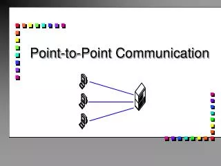
Simulation of an Optical Fiber Point to Point Communication link using Simulink. By Nihal Shastry Uday Madireddy Nitin Ravi. Overview of Project. Current scenario Where our project fits in Comparison of modulation techniques QAM MPSK EXTERNAL MODULATION

E N D
Simulation of an Optical Fiber Point to Point Communication link using Simulink By Nihal Shastry Uday Madireddy Nitin Ravi
Overview of Project • Current scenario • Where our project fits in • Comparison of modulation techniques QAM MPSK EXTERNAL MODULATION • Applications • Future scope
What is QAM? • QAM can be the expanded as Quadrature Amplitude Modulation • A popular digital modulation technique in which both phase and amplitude are varied • It was basically developed to overcome constraints of complex AM or PM • It can transmit more bits per second • It also makes use of minimum Bandwidth
Phase Shift Keying • Principle - Changes the phase of the carrier in step with the digital message. • Use of a different phase for a “0” and a “1”. • A “1” signal is denoted by φ1. • A “0” signal is denoted by φ1 + 180°. • Quaternary Phase shift keying • Binary inputs – 00, 01, 10, 11 • QPSK output phase -- 0°, 90°, 180°, 270°. • Differential Phase Shift Keying • Information obtained as the difference in phase between two successive signals. • Modulating signal is not the binary code but the code that records the changes in the binary code.
Optical communication link – QPSK modulation • QPSK- Quadrature / Quaternary Phase Shift Keying • Digital modulation technique • M-ary Encoding technique where M = 4 • 4 different input conditions, 4 output phases possible for a single carrier frequency.
QPSK • Four phases:- 0°, 90°, 180°, 270°. • Two symbols per bit can be transmitted (00, 01, 10, 11). • Each symbol’s phase compared with respect to the previous symbol.
External Modulation • Currently preferred over any other form of modulation • Done using an MZIM • Phase difference produced in the beam
HEAD TO HEAD • QAM: • Digital information contained in both amplitude and phase of the transmitted carrier • Susceptible to interfering signals • Greater bandwidth efficiency. More bits transferred(4bits/cycle) • QPSK: • Digital information - phase of the transmitted signal. • Easy to implement and has good resistance to noise. • In the receiver end local oscillator to be tuned to the I/P signal. • Oscillator experiences drift in freq and phase and hence tuning is tough • Overcome by sending a pilot wave for synchronization • Bandwidth Efficiency is around 2 bits per cycle. • DPSK: • Simple to implement • Larger data transmission capability (40 Gbits/Sec) • Has maximum transmission distance when compared to other schemes.
Applications • Can be used for simulating theoretical systems inexpensively • Any distance, bit rate and data pulse can be simulated • All parameters are completely user defined • Completely customizable
References • www.intel.com • Electronic Communications systems – Wayne Tomasi • www.ee.buffalo.edu/faculty/paololiu/413/ • binary.engin.brown.edu/lecture/Denmark/ • Noise analysis for optical fiber communication systems -Alper Demir- Istanbul • Transmission Line laser modeling of semi conductor laser amplified optical communication systems -A.J lowery-IEE proceedings V 139 #3 June 1992
Design of analog and digital data transmission filters- Hussein, Baher -IEEE trans on circuits and systems Vol# 40 #7 1993 • Frequency chirping in external modulators- Fumio Koyama IEEE J of light wave technology Vol #6 #1 Jan 1998 • Design of optical communication data links- P.K. Pepeljugoski et all- IBM J of Res. and Dev. Vol #47 No.2/3 2003 • A time domain optical transmission system simulation package accounting for non linear and polarization- related effects in a fiber- Andrea Carena et all- IEEE J on selected areas in comm. V #15 #4 May 1997