Download

1 / 73
760 likes | 1.04k Views
Stability Analysis of Non-linear Control Systems using Genetic Programming. LPPD Weekly Seminar. Benyamin Grosman. 4/30/2008. Outline. Short introduction to genetic programming. Steady-state modeling Dynamic modeling & NMPC Lyapunov stability and Lyapunov functions .

E N D
Stability Analysis of Non-linear Control Systems using Genetic Programming LPPD Weekly Seminar Benyamin Grosman 4/30/2008
Outline Short introduction to genetic programming. Steady-state modeling Dynamic modeling & NMPC Lyapunov stability and Lyapunov functions. Optimal Nonlinear control synthesis
Genetic Programming Automatic model generation by evolutionary mechanism. Model structure and its corresponding parameters are simultaneously optimized. Advantages • Analytical form of model is automatically generated from a library of mathematical operators/functions. • The library can be expanded to include a priori information about the process under consideration. • Very useful for poorly understood complex processes Disadvantages • Effectiveness is suspect for many input variables. Use of a quick and efficient variable selection algorithm can alleviate this problem to a large extent.
Main Components of a GP • The following operators are required • Population initialization, to seed the initial population with solution candidates; • An evaluation procedure, playing the role of the environment, which rates solution according to fitness; • A selection procedure, to pick a subset of more successful solution for reproduction; • Reproduction,recombination and mutation operators, which are rules defining how successful parents are recombined to form children. • Appropriate termination criteria need to be defined.
GP: Chromosomal Representation × + A B C Main branches Tree-structure model representation. Allows for heterogeneous populations of models with different complexities. Root of tree (A+B)×C
GP: Solution Evaluation Fitness based on data set used for parameter optimization Fitness computed using verification data Plays the role of the environment. Rates the “fitness” of each solution in the population. In our GP (Grosman and Lewin, 2005), the fitness of a model is assessed using the function:
GP: Solution Evaluation and of the penalty on the complexity of the model Slope of the penalty Freedom of expansion Number of branches Constant updated each generation to match the complexity of the best current solution
GP: Solution Evaluation Imposing adaptive penalty on the complexity of the model
GP: Reproduction -Crossover × × + + + + ÷ A A B B E C E C F F F F ÷ Cross-fertilization of chromosomes of successful parents. The new offspring are added to the solution pool.
GP: Reproduction -Mutation × × × ÷ × × × + + + + + + + + A A A A A A A A B B B B B B B B C C C C C C C × log C Adds new features by random perturbation.
GP: Reproduction -Permutation ÷ ÷ ÷ + + + A A A B B B C C C Adds new features by random switching of model branches.
The hidden model McKay’s best result: y = u1u22(3.0007−0.1506u2+0.1885u22)+2.99u3 RMS=0.47 Our GP best result: y = 0.0259u1 exp(5.555×u24.596 exp(−1.739u2))+3.004u3 RMS=0.017 Steady-state modeling Five inputs(u1-u5) where selected to augment between 0 and 1 McKay et al (1997)
Dynamic identification and NMPC We try to identify the general nonlinear MISO model: And use it in a General MPC schema
Dynamic identification and NMPC Case study - Karr type liquid liquid exchange column:
Dynamic identification and NMPC The system has two outputs: 1. The dispersed phase effluent concentration, Xout 2. The column holdup And three inputs: Qcin, Qdin, f
Dynamic identification and NMPC model identified: The NMPC controller was compared to a decoupled controller:
Stability-Some system definitions A dynamic system is said to be autonomous if f does not depend explicitly on time An equilibrium point of the system , x = x*, is one that satisfies:
Stability Definition Definition: the equilibrium 0 is stable if, for each ε>0 and each , there exists a δ= δ(ε,t0) such that: (Vidyasager, 1993)
Lyapunov functions and theDirect Method • If, in a ball BR0, there exists a scalar function • with continuous first partial derivatives such that • * is positive definite • * is negative semi-definite • then the equilibrium point is stable
Main Drawback ofthe Direct method The method suffers from common difficulty of finding a Lyapunov function for given system. Since there is no generally effective approach for finding Lyapunov functions, one has to resort to trial-and-error, experience, and intuition to search for an appropriate Lyapunov function (Slotine Li, 1991)
Domain of attraction This system has a stable domain of attraction of the radius of The nature of the orbits are due to their pure real eigenvalues
The Domain of Attraction • Unfortunately, even if the Lyapunov conditions for asymptotic stability are fulfilled in a specified closed region around the equilibrium point, this does not guarantee that this region is included in the domain of attraction This forces us to employ the concept of level-sets…
Level sets • We need to recognize the highest level-set of the Lyapunov function that is entirely included in the domain that satisfies the Lyapunov conditions This level set defines an area included in the domain of attraction
Level sets • Furthermore, if this level set is not connected, then the minimum radius from the borders of this level-set to the origin belongs to the connected set that includes the origin
Finding Lyapunov function using Genetic Programming The first thing that has to be established before developing a GP is to definite what constitutes the fittest function. Let’s define when a candidate is a potential Lyapunov function…
Finding Lyapunov functions using Genetic Programming (Cont’d) A two step optimization is implemented: • The extent that the Lyapunov conditions are fulfilled is checked in a relatively small domain. • The maximal level set and its minimum radius from the origin are detected on a predefined area to set the final optimization grade.
Finding Lyapunov functions using Genetic Programming (Cont’d) Initial ball Non positive values of the candidate in the initial ball Positive values of the candidate in the initial ball Step I:
Finding Lyapunov functions using Genetic Programming (Cont’d) Step I optimization function Non positive values of the candidate in the initial ball Positive values of the candidate in the initial ball
Finding Lyapunov functions using Genetic Programming (Cont’d) + The black plus represents a domain of positive v(x) values while the cross black points identify a domain of negative values of the derivative of v(x) with respect to time Their superposition defines the domain that satisfies the Lyapunov conditions. • Step II:
Finding Lyapunov functions using Genetic Programming (Cont’d) Because the minimum radius of the level set borders must belong to the connected set that includes the origin, it provides the most reliable index of the quality of a candidate's predicted domain of attraction. Noting that the score appropriate for the GP is a fitness value in the range between zero and unity, we define fitness as: Minimum radius to the origin GP score
Vannelli and Vidyasagar • This method is based on an iterative procedure for finding what they call maximal Lyapunov functions, which are rational by their nature and are the result of the division of two multivariable polynomials. • In the following, we compare our results with those of Vannelli and Vidyasagar; the first two example are two-dimensional and the last one is three-dimensional
Vannelli and Vidyasagar (Cont) Example I
Vannelli and Vidyasagar (Cont) Example II
Vannelli and Vidyasagar (Cont) Example III
HAMILTON-JACOBI-BELLMAN Nonlinear control systems are of the general form: Let us express a general cost function General cost function The cost of getting there
HAMILTON-JACOBI-BELLMAN For a small shift in time, we can rewrite the former equation into: We can assume knowing the optimal cost from any point in space
HAMILTON-JACOBI-BELLMAN The Lyapunov equation
HAMILTON-JACOBI-BELLMAN Again, for a small shift in time, we can rewrite the former equation into: We look for the move u in the next small time interval that will minimize J(x)
HAMILTON-JACOBI-BELLMAN Example with a standard cost function: This results in the following optimal control law:
HJB and GP From the moment the explicit control law is obtained the problem seems to be solved - but what should be the new GP cost function? The simplest way is using the same cost function we used to obtain a maximum domain of attraction - but this may result in a very large domain of attraction obtained by unreasonably large control moves
HJB and GP A better approach will take into consideration the solution of the HJB while trying to maximize the domain of attraction
HJB and GP The initial small predefined area The domain of attraction minimum radius The normalized Value of the HJB equation in the domain of attraction
Normalized CSTR where:
Normalized CSTR . It is desired to maintain the system at the unstable equilibrium point by manipulating the feed-flow rate F. Moreover, the feed-flow F is under the following constrains