Download
1 / 18
442 likes | 3.34k Views
THEORY OF CONSUMER BEHAVIOUR. The principle assumption upon which the theory of consumer behavior and demand is built is: a consumer attempts to allocate his/her limited money income among available goods and services so as to maximize his/her utility (satisfaction).

E N D
THEORY OF CONSUMER BEHAVIOUR The principle assumption upon which the theory of consumer behavior and demand is built is: a consumer attempts to allocate his/her limited money income among available goods and services so as to maximize his/her utility (satisfaction).
THEORY OF CONSUMER BEHAVIOUR Useful for understanding the demand side of the market. Utility - amount of satisfaction derived from the consumption of a commodity ….measurement units utilities
THEORY OF CONSUMER BEHAVIOUR • Utility Concepts: • The Cardinal Utility Theory (TUC) • Utility is measurable in a cardinal sense • cardinal utility - assumes that we can assign values for utility, (Jevons, Walras, and Marshall). E.g., derive 100 utils from eating a slice of pizza • The Ordinal Utility Theory (TUO) • Utility is measurable in an ordinal sense • ordinal utility approach - does not assign values, instead works with a ranking of preferences. (Pareto, Hicks, Slutsky)
The Cardinal Approach Nineteenth century economists, such as Jevons, Menger and Walras, assumed that utility was measurable in a cardinal sense, which means that the difference between two measurement is itself numerically significant. UX = f (X), UY = f (Y), ….. Utility is maximized when: MUX / MUY = PX / PY
The Cardinal Approach • Total utility (TU) - the overall level of satisfaction derived from consuming a good or service • Marginal utility (MU) additionalsatisfaction that an individual derives from consuming an additional unit of a good or service. Formula : MU = Change in total utility Change in quantity = ∆ TU ∆ Q
The Cardinal Approach • Law of Diminishing Marginal Utility (Return) = As more and more of a good are consumed, the process of consumption will (at some point) yield smaller and smaller additions to utility • When the total utility maximum, marginal utility = 0 • When the total utility begins to decrease, the marginal utility = negative (-ve)
The Cardinal Approach • TU, in general, increases with Q • At some point, TU can start falling with Q (see Q = 5) • If TU is increasing, MU > 0 • From Q = 1 onwards, MU is declining principle of diminishing marginal utility As more and more of a good are consumed, the process of consumption will (at some point) yield smaller and smaller additions to utility
Consumer Equilibrium • So far, we have assumed that any amount of goods and services are always available for consumption • In reality, consumers face constraints (income and prices): • Limited consumers income or budget • Goods can be obtained at a price
Consumer Equilibrium • Consumer’s objective: to maximize his/her utility subject to income constraint • 2 goods (X, Y) • Prices Px, Py are fixed • Consumer’s income (I) is given
Consumer Equilibrium • Marginal utility per price additional utility derived from spending the next price (RM) on the good • MU per RM = MU P
Consumer Equilibrium • Optimizing condition: • MUx = MUy PxPy • If MUxMUy PxPy • spend more on good X and less of Y
The Ordinal Approach • Economists following the lead of Hicks, Slutsky and Pareto believe that utility is measurable in an ordinal sense--the utility derived from consuming a good, such as X, is a function of the quantities of X and Y consumed by a consumer. • U = f ( X, Y )
Ordinal Utility Theory (TUO) • Can be measured in qualitative, not quantitative, but only lists the main options (indifference curves & budget line). • Rational human beings will choose to maximize the utility by selecting the highest utility • Difference consumers, difference utilities.
INDIFFERENCE CURVE (IC) • Curve where the points represent a combination of items when the consumer at indifference situation (satisfaction). • Axes: both axes refer to the quantity of goods • For the combination that produces a higher level of satisfaction, the curves shift to the right (IC2) from the first curve (IC1) • In contrast, the curves shift to the left (IC-1)
PROPERTIES OF INDIFFERENCE CURVE • Downward sloping from left to right: This shows an increase in quantity of certain good. • Convex to the origin: the marginal rate of substitution (MRS) decreased • MRS = quantity of goods Y willing to substitute to obtain one unit of goods X & this substitution is to maintain its position at the same level of satisfaction • Do not cross (intersect): consumer preferences transitive • Eg : Quantities X and Y for the combination of A> a combination of B; utility A> B * When cross = C, so the utility A = C & B = C; utility A = B = C. This is not transitive as above * • Different ICs show different level of satisfaction. Far from the origin, the higher the satisfaction.
Budget line (BL) • Line showing all combinations of items can be purchased for a particular level of income (M) ; M =PxQx + PyQy • The slope depends on the prices of goods X and Y, the slope = Px/Py • Slope -ve: to use more goods X, Y should reduce & vice versa • In the X-axis, when the quantity Y = 0, all M used to purchase X; M = PxQxQx =M/Px • At the Y axis, when the quantity X = 0, all M used to purchase Y; M = PyQyQy =M/Py
EFFECTS OF PRICE CHANGES ON THE BUDGET LINE • When price of good X increases, the quantity of good X is reduced (by maintaining the quantity of Y) & vice versa. Points on the X axis shifted to the left (a small quantity of X) • When the price of Y increases, the quantity Y is reduced (by maintaining the quantity of X) & vice versa Point on Y axis move to the bottom (small quantity in Y)
CONSUMER EQUILIBRIUM • With income (M) some combination of goods that consumers choose the highest satisfaction • Satisfied the same curves and budget lines are connected • The point where the curve IC and BL tangent • Slope IC = BL • Consumer choice influenced by income • Increased income, increased consumer equilibrium point