Download
1 / 48
660 likes | 1.2k Views
Economic Models of Credit Risk Lectures 10 & 11. Credit Risk Modeling. Based on Risk Management, Crouhy, Galai, Mark, McGraw-Hill, 2000. (Kealhofer / McQuown / Vasicek). The Contingent Claim Approach - Structural Approach: KMV . The Option Pricing Approach: KMV.

E N D
Economic Models of Credit Risk Lectures 10 & 11 Credit Risk Modeling Based on Risk Management, Crouhy, Galai, Mark, McGraw-Hill, 2000
(Kealhofer / McQuown / Vasicek) The Contingent Claim Approach - Structural Approach: KMV
The Option Pricing Approach: KMV KMV challenges CreditMetrics on several fronts: 1. Firms within the same rating class have the same default rate 2. The actual default rate (migration probabilities) are equal to the historical default rate (migration frequencies) • Default rates change continuously while ratings are adjusted in a discrete fashion. • Default rates vary with current economic and financial conditions of the firm.
The Option Pricing Approach: KMV KMV challenges CreditMetrics on several fronts: 3. Default is only defined in a statistical sense without explicit reference to the process which leads to default. • KMV proposes a structural model which relates default to balance sheet dynamics • Microeconomic approach to default: a firm is in default when it cannot meet its financial obligations • This happens when the value of the firm’s assets falls below some critical level
The Option Pricing Approach: KMV KMV’s model is based on the option pricing approach to credit risk as originated by Merton (1974) 1. The firm’s asset value follows a standard geometric Brownian motion, i.e.: dV = m + s t dt dZ t V t ì ü s 2 = m - + s Z V V exp ( ) t t í ý 0 t t 2 î þ
Assets Liabilities / Equity Debt: Bt (F) Risky Assets: Vt Equity: St V V Total: t t The Option Pricing Approach: KMV 2. Balance sheet of Merton’s firm
The Option Pricing Approach: KMV Equity value at maturity of debt obligation: ( ) = - S max V F , 0 T T Firm defaults if < V F T with probability of default (“real world” probability measure) æ ö æ ö s 2 V ç ÷ + ç m - ÷ Ln T 0 ç ÷ F 2 ç ÷ è ø ( ) ( ) < = Z < - = - 0 P V F P N d ç ÷ T T 2 s T ç ÷ ç ÷ è ø
ì í î The Option Pricing Approach: KMV 3. Probability of default (“real world” probability measure) • Distribution of asset values at maturity of the debt obligation Assets Value ü æ ö s 2 = m - + s Z ç ÷ ý V V exp T T T O è ø T 2 þ m = T E ( ) V e V O T V T V 0 F Probability of default Time T
- rT B + P = Fe 0 0 The Option Pricing Approach: KMV Bank’s pay-off matrix at times 0 and T for making a loan to Firm ABC and buying a put on the value of ABC Time 0 T £ Value of Assets V V F V F > 0 T T Bank’s Position: · -B F V make a loan 0 T · -P F - V O buy a put 0 T Total -B -P F F 0 0 Corporate loan = Treasury bond + short a put
Po = f ( Vo, F, sv, r, T ) (Black-Scholes option price) • Bo = Fe-rT - Po • So = Vo - Bo (assuming markets are frictionless) • Bo = Fe-YTTwhere YT is yield to maturity • Probability of Default = g (Vo, F, sv, r, T) = N ( - d2 ) • (“risk neutral” probability measure) 6Conditional recovery when default = VT KMV: Merton’s Model Firm ABC is structured as follows: Vt = Value of Assets (at time t) St = Value of Equity Bt = Value of Debt (zero-coupon) F = Face Value of Debt
KMV: Merton’s Model Problem: Vo ( say =100 ), F ( say = 77 ), sv ( say = 40% ), r ( say =10% ) and T ( say = 1 year) Solve for Bo,So,YT and Probability of Default
KMV: Merton’s Model ` Solution: P0( = 3.37) ® Bo( = 66.63) ® So( = 33.37) ® YT ( =15.6%) ®PT ( = 5.6%) æ ö F = ® P = - ç ÷ = - = - Y L Y r = - rT P f ( V , T ) S V B B Fe P K T N T T o o o o o o o è ø B o Note: In solving for P0 we get Probability of Default ( = 24.4% )
The Option Pricing Approach: KMV P = - Default spread ( ) for corporate debt ( For V0 = 100, T = 1, and r = 10% ) Y r T T s 0.05 0.10 0.20 0.40 LR 0.5 0 0 0 1.0 0.6 0 0 0.1% 2.5% 0.7 0 0 0.4% 5.6% 0.8 0 0.1% 1.5% 8.4% 0.9 0.1% 0.8% 4.1% 12.5% 1.0 2.1% 3.1% 8.3% 17.3% - rT Fe Leverage ratio: = LR V 0
KMV: EDFs (Expected Default Frequencies) 4. Default point and distance to default Observation: Firms more likely to default when their asset values reach a certain level of total liabilities and value of short-term debt. Default point is defined as DPT=STD+0.5LTD STD-short-term debt LTD- long-term debt
KMV: EDFs (Expected Default Frequencies) Default point (DPT) Probability distribution of V Asset Value Expected growth of assets, net E(V) 1 V0 DD DPT = STD + ½ LTD Time 1 year 0
KMV: EDFs (Expected Default Frequencies) Distance-to-default (DD) DD- is the distance between the expected asset value in T years, E(VT) , and the default point, DPT, expressed in standard deviation of future asset returns:
KMV: EDFs (Expected Default Frequencies) 5. Derivation of the probabilities of default from the distance to default EDF 40 bp 4 6 1 2 5 3 DD KMV also uses historical data to compute EDFs
- 1 , 200 800 = = DD 4 100 KMV: EDFs (Expected Default Frequencies) Example: V0 = 1,000 Current market value of assets: Net expected growth of assets per annum: Expected asset value in one year: Annualized asset volatility, Default point 20% : V1 = V0(1.20) = 1,200 sA 100 800 Assume that among the population of all the firms with DD of 4 at one point in time, e.g. 5,000, 20 defaulted one year later, then: 20 = = = EDF 0 . 004 0 . 4% or 40 bp 1 year 5 , 000 The implied rating for this probability of default is BB+
KMV: EDFs (Expected Default Frequencies) Example:Federal Express ($ figures are in billions of US$) November 1997 February 1998 Market capitalization (S0 ) (price* shares outstanding) Book liabilities Market value of assets (V0 ) Asset volatility Default point Distance to default (DD) EDF $ 7.8 $ 4.8 $ 12.6 15% $ 3.4 12.6-3.4 0.15·12.6 0.06%(6bp) $ 7.3 $4.9 $ 12.2 17% $ 3.5 12.2-3.5 0.17·12.2 0.11%(11bp) = 4.9 = 4.2 º A º AA
KMV: EDFs (Expected Default Frequencies) 4. EDF as a predictor of default EDF of a firm which actually defaulted versus EDFs of firms in various quartiles and the lower decile. The quartiles and decile represent a range of EDFs for a specific credit class.
KMV: EDFs (Expected Default Frequencies) 4. EDF as a predictor of default EDF of a firm which actually defaulted versus Standard & Poor’s rating.
KMV: EDFs (Expected Default Frequencies) 4. EDF as a predictor of default Assets value, equity value, short term debt and long term debt of a firm which actually defaulted.
Credit Suisse Financial Products IV The Actuarial Approach: CreditRisk+
The Actuarial Approach: CreditRisk+ In CreditRisk+ no assumption is made about the causes of default: an obligor A is either in default with probability PA, or it is not in default with probability 1-PA. It is assumed that: • for a loan, the probability of default in a given period, say one month, is the same for any other month • for a large number of obligors, the probability of default by any particular obligor is small and the number of defaults that occur in any given period is independent of the number, of defaults that occur in any other period
The Actuarial Approach: CreditRisk+ Under those circumstances, the probability distribution for the number of defaults, during a given period of time (say one year) is well represented by a Poisson distribution: where m = average number of defaults per year æ ö å m m = P It is shown that can be approximated as ç ÷ A è ø A
CreditRisk+: Frequency of default events One year default rate Credit Rating Average (%) Standard deviation (%) Aaa 0.00 0.0 Aa 0.03 0.1 A 0.01 0.0 Baa 0.13 0.3 Ba 1.42 1.3 B 7.62 5.1 m Note, that standard deviation of a Poisson distribution is . For instance, for rating B: . m = = 7 . 62 2 . 76 versus 5 . 1 CreditRisk+ assumes that default rate is random and has Gamma distribution with given mean and standard deviation. Source: Carty and Lieberman (1996)
CreditRisk+: Frequency of default events Probability Excluding default rate volatility Including default rate volatility Number of defaults Source: CreditRisk+ Distribution of default events
CreditRisk+: Loss distribution • In CreditRisk+, the exposure for each obligor is adjusted by the anticipated recovery rate in order to produce a loss given default (exogenous to the model)
CreditRisk+: Loss distribution 1. Losses (exposures, net of recovery) are divided into bands, with the level of exposure in each band being approximated by a single number. Notation A Obligor Exposure (net of recovery) LA PA Probability of default lA=LAxPA Expected loss
CreditRisk+: Loss distribution Example: 500 obligors with exposures between $50,000 and $1M (6 obligors are shown in the table) Round-offexposure(in $100,000) Exposure ($)(loss given default) Exposure(in $100,000) Obligor Band L n n A j j j A 1 150,000 1.5 2 2 2 460,000 4.6 5 5 3 435,000 4.35 5 5 4 370,000 3.7 4 4 5 190,000 1.9 2 2 6 480,000 4.8 5 5 The unit of exposure is assumed to be L=$100,000. Each band j, j=1, …, m, with m=10, has an average common exposure: vj=$100,000j
CreditRisk+: Loss distribution In Credit Risk+ each band is viewed as an independent portfolio of loans/bonds, for which we introduce the following notation: Notation Common exposure in band j in units of L nj nj = $100,000, $200,000, …, $1M Expected loss in band j in units of L ej (for all obligors in band j) Expected number of defaults in band j mj ej = nj x mj mj can be expressed in terms of the individual loan characteristics
CreditRisk+: Loss distribution Number Band: of e m j j j obligors 1 30 1.5 (1.5x1) 1.5 2 40 8 (4x2) 4 3 50 6 (2x3) 2 4 70 25.2 6.3 5 100 35 7 6 60 14.4 2.4 7 50 38.5 5.5 8 40 19.2 2.4 9 40 25.2 2.8 10 20 4 (0.4x10) 0.4
µ µ å å n n = = = n G ( z ) P ( lossj nL ) z P ( n defaults ) z j j = = n 0 n 0 m - m n e j µ n å j n - m + m n z j = = z e G ( z ) j j j j n ! = n 0 CreditRisk+: Loss distribution To derive the distribution of losses for the entire portfolio we proceed as follows: Step 1: Probability generating function for each band. Each band is viewed as a portfolio of exposures by itself. The probability generating function for any band, say band j, is by definition: where the losses are expressed in the unit L of exposure. Since we have assumed that the number of defaults follows a Poisson distribution (see expression 30) then:
m m n - m + m å å z j m n j j - m + m z = Õ = G ( z ) e e j = = j j j 1 j 1 = 1 j CreditRisk+: Loss distribution Step 2: Probability generating function for the entire portfolio. Since we have assumed that each band is a portfolio of exposures, independent from the other bands, the probability generating function for the entire portfolio is just the product of the probability generating functions for all bands. m å m denotes the expected number of defaults for the entire portfolio. m where = j 1 j =
n 1 d G ( z ) = = P ( loss of nL ) | for n 1 , 2 ,... = z 0 n n ! dz j - ( ) ( ) v m = = = P 0 loss G 0 e e j j CreditRisk+: Loss distribution Step 3: loss distribution for the entire portfolio Given the probability generating function (33) it is straightforward to derive the loss distribution, since these probabilities can be expressed in closed form, and depend only on 2 sets of parameters: ej and nj . (See Credit Suisse 1997 p.26) e å e ( ( ) ) ( ) å = - j P loss of nL P loss of n v L j n £ j : v n j
Duffie-Singleton - Jarrow-Turnbull V Reduced Form Approach
Reduced Form Approach • Reduced form approach uses a Poisson process like environment to describe default. • Contrary to the structural approach the timing of default takes the bond-holders by surprise. Default is treated as a stopping time with a hazard rate process. • Reduced form approach is less intuitive than the structural model from an economic standpoint, but its calibration is based on credit spreads that are “observable”.
Reduced Form Approach Example: a two-year defaultable zero-coupon bond that pays 100 if no default, probability of default , LGD=L=60%. The annual (risk-neutral) risk-free rate process is : = r 12 % = p 0 . 5 ´ + ´ ´ 1 0 . 94 100 0 . 06 0 . 4 100 = = V 86 . 08 11 1 . 12 = r 8 % ´ + ´ ´ 0 . 94 100 0 . 06 0 . 4 100 = = V 87 . 64 12 1 . 1 = p 0 . 5 = r 10 % 2 ( ) ( ) ´ ´ + ´ ´ + ´ ´ + ´ ´ 0 . 5 0 . 94 V 0 . 06 0 . 4 V 0 . 5 0 . 94 V 0 . 06 0 . 4 V = V = 11 11 12 12 77 . 52 0 1 . 08
Reduced Form Approach “Default-adjusted” interest at the tree nodes is: 100 100 = - = = - = R 1 14 . 1 % R 1 16 . 2 % 12 11 87 . 64 86 . 08 ´ + ´ 0 . 5 86 . 08 0 . 5 87 . 64 = - = R 1 12 % 0 77 . 52 In all three cases R is solution of the equation ( ): D = t 1 1 1 [ ] = - l D + l D - ( 1 t ) t ( 1 L ) + D + D 1 R t 1 r t D + l D r t tL D = R t - l D + l D - 1 t t ( 1 L ) ® + l If , then , where is the risk-neutral expected loss rate, which can be interpreted as the spread over the risk-free rate to compensate the investor for the risk of default. l D ® R r L L t 0
é é é ù ù ù ê ê ê ú ú ú ë ë ë û û û Reduced Form Approach ( ) l t General case:is hazard rate, so that if denotes the time to default, the survival probability at horizon t is t t ò t > = - l Prob ( t ) E exp( ( s ) ds ) 0 ( ) l = l E is expectation under risk-neutral measure. For the constant we have: t t > = - l Prob ( t ) E exp( t ) ( ) The probability of default over the interval provided no default has happened until time t is: + D t , t t < t £ + D = l D Prob t t t ( t ) t (similar to the example above).
Reduced Form Approach Corporate curve ( ) R , r R t Yield spread = l L R Treasury curve r t Maturity Term structure of interest rates
Reduced Form Approach By modelling the default adjusted rate we can incorporate other factors which affect spreads such as liquidity: = + l + R r L l where l denotes the “liquidity” adjustment premium. if there is a shortage of bonds and one can benefit from holding the bond in inventory, if it becomes difficult to sell the bond. > l 0 < l 0 l l Identification problem : how to separate and in . Usually is assumed to be given. Implementations differ with respect to assumptions made regarding default intensity . L L L l
Reduced Form Approach How to compute default probabilities and l Example. Derive the term structure of implied default probabilities from the term structure of credit spreads (assume L=50%). Company X One-year Maturity Treasurycurve one-year forward credit t (years) forward rates spreads FS t (%) (%) (%) 1 5.52 5.76 0.24 2 6.30 6.74 0.44 3 6.40 7.05 0.65 4 6.56 7.64 1.08 5 6.56 7.71 1.15 6 6.81 8.21 1.40 7 6.81 8,47 1.65
P t Reduced Form Approach Forward Cumulative Conditional probabilities defauilt default Maturity of default probabilities probabilities (years) t p (%) (%) (%) l t t 1 0.48 0.48 0.48 2 0.88 1.36 0.88 3 1.30 2.64 1.28 4 2.16 4.74 2.10 5 2.30 6.93 2.19 6 2.80 9.54 2.61 3.30 12.52 2.99 7 l = = l ´ = 2 . 16 FS L 1 . 08 % For example, for year 4: , then 4 4 4 ( ) Cumulative probability: = + - ´ l = P P 1 P 4 . 74 4 3 3 4 ( ) Conditional probability: = - ´ l = p 1 P 2 . 10 4 3 4
Reduced Form Approach • Generalizations: • Intensity of the default is modeled as a Cox process (CIR model), conditional on vector of state variables , such as default free interest rates, stock market indices, etc. • where is a standard Brownian motion, is the long-run mean of is mean rate of reversion to the long-run mean, is a volatility coefficient. • Properties: • , • Conditional survival probability , where • and are known time-dependent functions of time, • The volatility of is ( ) l t ( ) X t ( ) ( ( ) ) ( ) ( ) l = q - l + l s d t k t dt t dB t , ( ) q l B t s k ( ) l ³ t 0 ( ) ( ) ( ) ( ) a - + b - l = t s t s t p t , s e b a ( ) ( ) ( ) ( ) = b - s l p t , s s t t p t , s
l (b.p.) 0 Years Reduced Form Approach • Generalizations: • Intensity of the default can be modeled as a jump process: • where , - cumulative jumps by at Poisson arrival times, is mean arrival rate, is mean jump size. ( ) l t ( ) ( ( ) ) ( ) l = q - l + d t k t dt dZ t , ( ) ( ) ( ) t = - g Z t N t Jt N t g J Take jumps sizes to be, say, independent and exponentially distributed.
Reduced Form Approach • Generalizations: • Risk free spot rate is modeled as one factor extended Vasicek process. • where , , are similar to parameters in CIR model, • is a function defined from current term structure of interest rates. is correlated with Brownian motion of the default intensity process. • Closed form solutions for the bond prices. ( ) r t ( ) ( ( ) ( ) ) ( ) = q - + s dr t k t r t dt dB t , 1 1 1 1 ( ) s B t k 1 1 1 ( ) q t 1 ( ) B t 1
Reduced Form Approach • Inputs : • the term structure of default-free rates • the term structure of credit spreads for each credit category • the loss rate for each credit category • Model assumptions : • zero correlations between credit events and interest rates • deterministic credit spreads as long as there are no credit events • constant recovery rates