Download
1 / 52
520 likes | 667 Views
Light scalar nonets in pole-dominated QCD sum rules. T. Kojo (Kyoto Univ.). D. Jido (YITP). 4 -quark picture leads the favorable prescription (Jaffe, 1977). 2 - quark picture has the difficulty:. The assignment assuming the ideal mixing:. wrong ordering.

E N D
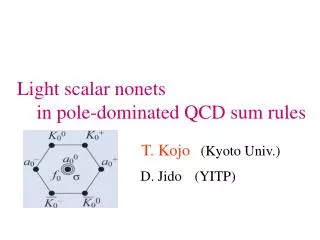
Light scalar nonets in pole-dominated QCD sum rules T. Kojo (Kyoto Univ.) D. Jido(YITP)
4 -quark picture leads the favorable prescription (Jaffe, 1977) 2 - quark picture has the difficulty: The assignment assuming the ideal mixing: wrong ordering To obtain JP = 0+state, P-wave excitation (~500MeV) is needed. Natural explanation for mass ordering & decay mode & width The masses exceed ~ 1 GeV. Possible strong diquark correlation (?) → mass < 1 GeV Light scalar nonets~ candidates of exotic hadrons 0 1/2 1 0 isospin: 600 ? 800 ? 980 980 mass (MeV): width: broad broad narrow narrow
The purpose of my talk The purpose of my talk is: to provide the information to consider the relevant constituents possible mixing with 2q & 2qG for light scalar nonets, using theQCD Sum Rules. We already know the 2q operator analysis fails to reproduce the lightness of light scalar nonets. Therefore, we perform the QSR analysis using the tetraquark operators.
2, Basics of QCD Sum Rules & typical artifacts in the application to the exotics
OPE hard soft Borel window ? small large OPE bad OPE good QCD Sum Rules (QSR)
1, Set the Borel window for each Sth : constraint for OPE convergence constraint for continuum suppression highest dim. / whole OPE < 10 % pole / whole spectral func. > 50 % Mmin < M <Mmax 2, Plot physical quantities as functions of M2: effective mass: peak like structure stability against M variation Eth 3, Select Sth to give the good stability against the variation of M. E Procedures for estimating the physical quantities
1.Good OPE convergence 2. Good continuum suppression 3. small M2-dependence M2small ? QSR for Exotics Difficulty to analyze Exotics When quark number of operator is large, realizing the conditions 1, 2 becomes extremely difficult. Indeed, in most of the previous works, OPE convergence is not good, and pole / whole contributionin the spectral integral isless than ~20 %! R.D.Matheus and S.Narison, hep-ph/0412063 In the M2 region where pole ratio is too small, the artificial stability of the physical parameters emerges! ( Even in the meson and baryon cases ) To avoid the artificial stability, we must estimate the physical values in the Borel window.
Eth Eth dim 0 ~ 6 pseudo peak ! E dim 8 ~ 12 E QSR artifact ~ pseudo peak artifact dim 10 ~ 12 dim 0 ~ 8 : outside of the Borel window Spectral function dim 0 ~ 6 dim 8 ~ 12
mass residue These artifacts are easily rejected by Borel window. & inclusion of higher dimension (> 6) terms. Pseudo peak artifact ~ Impact on physical quantities spectral function pole dominance
output: mass ? width = 400 MeV Impact of width on physical quantities effective mass: example:Breit-Wigner form (pole mass = 600 MeV) input: Breit-Wigner We will estimate the physical quantities considering the error from width effects.
most important for meaningful estimation Borel window well-isolated peak-like structure weak M – dep. (not strongly affected by background) weak Eth – dep. well-separated from threshold OPE: up to dim12within vacuum saturation Must be calculated to find the Borel window ! Calculation Set up of the operator: Linear combination: θwill be chosen to achieve:
large pure singlet: num. of annihilation diagrams pure octet: small Annihilation diagrams ~ Flavor dependence 2q - 4q, 2qG - 4q mixing The number of annihilation diagrams strongly depends on the flavor. & cyclic diquark base:
mass: 0.7 ~ 0.85 GeV mass: 0.6 ~ 0.75 GeV Eth: 1.0 ~ 1.3 GeV Eth: 0.8 ~ 1.3 GeV May be broad, or small pole to background ratio Effective mass for pure singlet & octet ( in the SU(3) chiral limit )
Effective residue for pure singlet & octet smaller than singlet residue small pole to background ratio?
σ(600) f0(980) (preliminary) mass: 0.75 ~ 0.90 GeV mass: 0.6 ~ 0.75 GeV Eth: 0.9 ~ 1.3 GeV Eth: 1.1 ~ 1.5 GeV Effective mass plots for σ & f0
mass residue (×107 GeV8) No stability in the Borel window in the arbitrary θ a0 - channel Results for pure octet~ mass & residue for a0 a0(980) (preliminary) κ- channel shows almost same behavior.
Summary We perform the tetraquark op. analysis within the Borel window. To find the Borel window, the higher dim. calculation is inevitable to include the sufficient low energy correlation. Our analysises imply ( within our operator combinations ): The difference between singlet and octet originates from annihilation diagrams, 4q→2q or 4q→2qG. singlet channel has well-developed enhancement around E~ 0.7GeV. ( pole to background ratio may be large. ) octet channel may be strongly affected by low energy contaminations. ( pole to background ratio may be small or no pole. ) σ(600) and f0 (980) are more likely 4q rather than 2q state. ( in 2q op. case, their masses are ~ 1.0 - 1.3 GeV)
f0(1710) f0(1500) a0(1450) 2q?(L=1, S=1) K0*(1430) f0(1370) a0(980) f0(980) K0*(800) σ(600) (QQ)(QQ) (QQ)-(QQ) QQ QQ or GG vector, axial vector, tensor Scalar meson a2(1320) a1(1230) (L=1, S=1) (L=1, S=0) M (MeV) ρ(770) (L=0, S=1) singlet – octet mixing π(137) 1+ ¯(1) 0¯ ¯(1) 2+ ¯(1) 0+ ¯(1) 0+ (1/2) 0++(0) JPG(I) 1¯+(1) valence:
Pole dominance ~ importance of higher dim. terms Pole / Whole spectral function (σ- case ) +dim.8 Only after dim. 8 terms contributes, Mmaxbecomes large.
Annihilation diagrams have more importance split singlet & octet in 4q op. case than in 2q op. case. Annihilation diagrams increase in higher dim. terms. important especially in low energy region. Annihilation diagrams 2-quark 3-loop, α suppression 4-quark 4-loop, α suppression few loops, but equal to zero no suppression factor, few loops
4q-2q or 4q-2qG mixing qualitative behavior of dim 10, 12 dim 8 dim 6 dim 0 ~ 4 2qG mixing singlet 2q mixing octet E ~ 1 GeV ~ 2 GeV This 2qG mixing is turned out to be essential for the large correlation in low energy ~ 1 GeV.
4q-2q or 4q-2qG mixing essential for low energy enhancement contributes mainly 1~ 2 GeV enhancement can be interpreted as diquark-diquark correlation ? can be interpreted as 2q component above 1GeV ?
1, Jaffe: ( MIT bag model ) PRD15, (1976) 267 4 -quark picture leads the favorable prescription. Natural explanation for mass ordering & decay mode & width Possible strong diquark correlation (?) → mass < 1 GeV (due to strong chromo-magnetic interaction) Theoretical suggestions 1: 600 ? 800 ? 980 980 mass (MeV): ~500 ? ~ 400 ? width(MeV): 50 ~ 300 50 ~ 300
T. Barnes (estimate a0, f0 → 2γ width) PLB165, 434 (1985) a0 (2q) → 2γ : width ~ 1.6 keV ~ 8 ×exp. width a0 (KK) → 2γ: width ~ 0.6 keV ~ 3 ×exp. width f0 (KK) → 2γ: width ~ exp. width 3, Narison: ( phenomelogy with QCD sum rules cal. ) PRD73, 114024(2006) σ, f0 → strong 2q – glueball mixing. ( σ, f0 →2π width is too small in 4q case) a0 → 2q, not 4q ( a0 → 2γwidth is 1/1000 small in 4q case) κ → 2q ( strong interference with nonresonant background) Theoretical suggestions 2 & 3: 2, Weinstein & Isgur: ( 4-particle Shrodinger eq. ) qqqq bound states normally do not exist. PRL48, (1982) 659 a0(980), f0(980) → loosely KK bound states . ( but all cal. of width in QSR is suspicious)
s s d d d d Experimental results: PRL12, 121801(2002) PRL86, 770(2001) 1, Exp. at Fermi lab. ( E791 Collaboration ) PRL12, 765(2001) u ( no evidence for σ) W+ c s σ u ( mass = 478±17 MeV width = 324±21 MeV ) W+ c d κ ( mass = 797±62 MeV width = 410±130 MeV )
Lattice: Kentucky group Scalar meson overlap fermion (χ-symmetry) volume dep. f0(1710) a0(1450), K0(1430) → 2q f0(1500) a0(1450) σ(600) → 4q K0*(1430) f0(1370) UK QCD group Nf=2 sea quark (partially quenched) a0(980) f0(980) M (MeV) No KK, using (ud) picture a0(980) → reproduced within 2q? K0*(800) Scalar collaboration σ(600) dynamical fermion (including glueball mixing) disconnected diagram dominate (σ case) light σ
simple parametrization , … Dispersion relation, OPE, quark-hadron duality QCD side Hadronic side spectral function Operator Product Expansion ? (OPE) soft q q hard sum of local operators information of QCD vacuum
OPE bad OPE good , Borel window small large Within the Borel window, we represent mass & residue as functions of the unphysical expansion parameter M ( & physical value Sth ). should not depend on M physicalparameter Information of low energy we want to know Constraint for M Borel trans.
Eth Eth dim 0 ~ 6 pseudo peak ! E dim 8 ~ 12 E QSR artifact ~ pseudo peak artifact : outside of the Borel window Spectral function dim 0 ~ 6 dim 8 ~ 12
1, Set the Borel window for each Sth : constraint for OPE convergence constraint for continuum suppression highest dim. / whole OPE < 10 % pole / whole spectral func. > 50 % Mmin < M <Mmax Procedures for estimating the physical quantities 2, Plot the physical quantities as functions of M2. If these quantities heavily depend on M2 in the Borel window, 1-pole + continuum approximation is bad.. We must consider another possibilities: 2 or 3 poles, smooth function for the scattering states and so on. 3, Select Sth to give the best stability against the variation of M.
( up to dim. 6 ) -meson case 1.2 3 1.0 0.8 Borel window 0.6 1 2 0.4 0.4 0.6 0.8 1.0 1.2 1.4 Note for physical importance of higher dim. terms of OPE: 750~790 770 2.3~2.5 2.36 Only after including dim.6 terms of OPE (including low energy correlation) , stability emerges in the Borel window. Dim.6 terms are responsible for the ρ-A1 mass splitting. (Without dim.6 terms, OPE forρand A1 give the same result.) Example when QSR is workable:
1.Good OPE convergence 2. Good continuum suppression 3. small M2-dependence M2small ? QSR for Exotics Difficulty to analyze Exotics When quark number of operator is large, realizing the conditions 1, 2 becomes extremely difficult. Indeed, in most of the previous works, OPE convergence is not good, and pole / whole contributionin the spectral integral isless than ~20 %! R.D.Matheus and S.Narison, hep-ph/0412063 In the M2 region where pole ratio is too small, the artificial stability of the physical parameters emerges! ( Even in the meson and baryon cases ) To avoid the artificial stability, we must estimate the physical values in the Borel window.
Eth Eth E dim 0 ~ 6 pseudo peak ! dim 0 ~ 6 dim 8 ~ 12 dim 8 ~ 12 E QSR artifact ~ pseudo peak artifact dim 10 ~ 12 dim 0 ~ 8 : outside of the Borel window
mass residue Pseudo peak artifact ~ examples spectral function pole dominance
OPE: up to dim12 within vacuum saturation Must be calculated to find the Borel window ! treatment of current quark mass: u, d-quark is treated in massless limit → x- rep. calculation s-quark mass is kept finite → p- rep. calculation resummation of the strange quark mass regulatemass ×divergence terms Calculation Set up of the operator: Linear combination: θwill be chosen to give the best stability in the Borel window.
assumption: ideal mixing Classification of nonets diquark base: singlet octet mass ordering: 600 800 980 980
large pure singlet: num. of annihilation diagrams pure octet: small Annihilation diagrams ~ Flavor dependence The number of annihilation diagrams strongly dependent on the flavor. & cyclic diquark base:
Criterions on selection of operators ( for stong low energy correlation, pole isolation ) 1, Sufficiently wide Borel window most important, well-satisfied for almost all θ 2, Weak M dependence necessary to avoid the contaminations below Eth 3, Weak threshold dependence necessary to avoid the contaminations from regions between “pole” and Eth 4, The sufficient strength of the effective residue necessary to avoid the truncated OPE error
Global analysis ~ θdependence Singlet residue mass θ Octet θ Singlet → better in Borel stability, larger residue Except some θ region, behavior is similar.
Effective mass plot ~ θ fixed to 7π/8 mass: 0.7 ~ 0.8 GeV mass: 0.6 ~ 0.75 GeV Eth: 1.0 ~ 1.3 GeV Eth: 0.8 ~ 1.3 GeV May be broad, or small pole to background ratio
Effective residue plot smaller than singlet residue
σ(600) f0(980) (preliminary) mass: 0.75 ~ 0.90 GeV mass: 0.6 ~ 0.75 GeV Eth: 0.9 ~ 1.3 GeV Eth: 1.1 ~ 1.5 GeV Effective mass plots for σ & f0
mass residue (×107 GeV8) No stability in the Borel window in the arbitrary θ a0 - channel Results for pure octet ~ mass & residue for a0 a0(980) (preliminary) κ- channel shows almost same behavior.
Experimental results: PRL12, 121801(2002) 1, Exp. at Fermi lab. ( E791 Collaboration ) PRL86, 770(2001) PRL12, 765(2001) Dalitz decay of D meson
Real world The states including the SU(3) singlet component: (preliminary) f0 (980): 0.75 ~ 0.90 GeV σ(600): 0.60 ~ 0.75 GeV The states including only the SU(3) octet component: no stability a0 (980): no stability κ(800): Summary We perform the tetraquark operator analysis within the Borel window. SU(3) chiral symmetric world Much stronger low energy correlation than 2-quark case → Borel window is easily found . octet: singlet: 0.70 ~ 0.85 GeV 0.6 ~ 0.75 GeV (stability not good) The difference comes from self-annihilation processes (diagrams). Some important effects associated with strange quark mass & hadronic threshold seem to be underestimated.
Resummation of current quark mass cut E E effective mass shifts to high energy side.
Mass × divergence example: ( dim.8 ) cut for spectral integral regulation for integral of Feynman parameter