Download
1 / 26
260 likes | 460 Views
LESSON 14 INVENTORY MODELS (DETERMINISTIC) RESOURCE CONSTRAINED SYSTEMS. Outline Resource Constrained Multi-Product Inventory Systems Fund constraint Space constraint. Resource Constrained Multiple Product Inventory Systems.

E N D
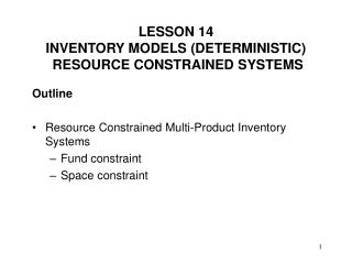
LESSON 14INVENTORY MODELS (DETERMINISTIC) RESOURCE CONSTRAINED SYSTEMS Outline • Resource Constrained Multi-Product Inventory Systems • Fund constraint • Space constraint
Resource Constrained Multiple Product Inventory Systems • So far, we have discussed inventory control models assuming that there is only one product of interest. • Often, there can be multiple products that may compete for the same resource such as fund, space, etc. • In such a case, the EOQ solutions may be satisfactory if the fund/space required by the EOQ solutions is less than that available. • However, The EOQ solutions cannot be implemented if the fund/space required by the EOQ solutions is more than that available.
Resource Constrained Multiple Product Inventory Systems • An important observation on the resource constrained models is the following: If the following ratio is the same for all products, an optimal order quantity of each product can be obtained by reducing its EOQ value by a constant multiplication factor. • We shall discuss two cases: • Fund constraint (satisfies the above condition) • Space constraint (may not satisfy the condition)
Fund ConstraintSame Interest Rate For All Products • If the same interest rate is applied on all products, the ratio is the same for all products. • Consequently, an optimal order quantity of each product can be obtained by reducing its EOQ value by a constant multiplication factor.
Fund ConstraintSame Interest Rate For All Products Steps 1. Compute the EOQ values and the total investment required by the EOQ lot sizes. If the investment required does not exceed the budget constraint, stop. 2. Reduce the lot sizes proportionately. To do this, multiply each EOQ value by the constant multiplier,
Example: Fund ConstraintSame Interest Rate For All Products Example 4: A vegetable stand wants to limit the investment in inventory to a maximum of $300. The appropriate data are as follows: Tomatoes Lettuce Zucchini Annual demand 1000 1500 750 (in pounds) Cost/pound $0.29 $0.45 $0.25 The ordering cost is $5 in each case and the annual interest rate is 25%. What are the optimal quantities that should be purchased?
Space Constraint • For each product, compute the following ratio • If the above ratio is the same for all products, a procedure similar to the one for the budget constraint may be applied. • Assume that the above ratios are different for different products (a reason may be that space requirement is not necessarily proportional to costs).
Space Constraint Steps 1. Compute the EOQ values and the total space required by the EOQ lot sizes. If the space required does not exceed the space constraint, stop. 2. By trial and error, find a value of such that the space required by the following lot sizes equals the space available:
Example: Space Constraint Example 5: A vegetable stand has exactly 500 square feet of space. The appropriate data are as follows: Tomatoes Lettuce Zucchini Annual demand 1000 1500 750 (in pounds) Space required 0.5 0.4 1 (square feet/pound) Cost/pound $0.29 $0.45 $0.25 The ordering cost is $5 in each case and the annual interest rate is 25%. What are the optimal quantities that should be purchased?
Example: Space Constraint q Trial value of Tomatoes Lettuce Zucchini Index, 1 2 3 i l Annual Demand, 1000 1500 750 i Ordering/Set-up Cost, 5 5 5 Ki Holding cost/unit/year, 0.0725 0.1125 0.0625 hi Space requirement/unit, 0.5 0.4 1 wi Lot sizes, Qi Space required Total space required Space available 500 Conclusion
Example: Space Constraint q Trial value of 0.1 Tomatoes Lettuce Zucchini Index, 1 2 3 i l Annual Demand, 1000 1500 750 i Ordering/Set-up Cost, 5 5 5 Ki Holding cost/unit/year, 0.0725 0.1125 0.0625 hi Space requirement/unit, 0.5 0.4 1 wi Lot sizes, 240.77 279.15 169.03 Qi Space required 120.39 111.66 169.03 Total space required 401.0748 Space available 500 Conclusion Decrease trial value (why?)
Example: Space Constraint q Trial value of 0.02 Tomatoes Lettuce Zucchini Index, 1 2 3 i l Annual Demand, 1000 1500 750 i Ordering/Set-up Cost, 5 5 5 Ki Holding cost/unit/year, 0.0725 0.1125 0.0625 hi Space requirement/unit, 0.5 0.4 1 wi Lot sizes, 328.80 341.66 270.50 Qi Space required 164.40 136.66 270.50 Total space required 571.5639 Space available 500 Conclusion Increase trial value (why?)
Example: Space Constraint q Trial value of 0.04287 Tomatoes Lettuce Zucchini Index, 1 2 3 i l Annual Demand, 1000 1500 750 i Ordering/Set-up Cost, 5 5 5 Ki Holding cost/unit/year, 0.0725 0.1125 0.0625 hi Space requirement/unit, 0.5 0.4 1 wi Lot sizes, 294.41 319.66 224.93 Qi Space required 147.21 127.86 224.93 Total space required 499.9997 Space available 500 Conclusion ?
READING AND EXERCISES Lesson 14 Reading: Section 4.8 , pp. 221-225 (4th Ed.), pp. 212-215 Exercise: 26, 28, p. 225 (4th Ed.), p. 215