College Physics Chapter 3 TWO-DIMENSIONAL KINEMATICS PowerPoint Image Slideshow
370 likes | 1.12k Views
College Physics Chapter 3 TWO-DIMENSIONAL KINEMATICS PowerPoint Image Slideshow. References. This material comes from Openstax College, which has published an online (and downloadable PDF) free physics textbook. http:// openstaxcollege.org/textbooks/college-physics

College Physics Chapter 3 TWO-DIMENSIONAL KINEMATICS PowerPoint Image Slideshow
E N D
Presentation Transcript
College Physics Chapter 3 TWO-DIMENSIONAL KINEMATICS PowerPoint Image Slideshow
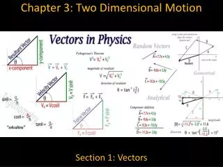
References • This material comes from Openstax College, which has published an online (and downloadable PDF) free physics textbook. • http://openstaxcollege.org/textbooks/college-physics • The corresponding textbook chapters are: • 3.2 Vector Addition and Subtraction: Graphical Methods • 3.3 Vector Addition and Subtraction: Analytical Methods • For practice, also see the PhET online simulation for vector addition: • http://phet.colorado.edu/en/simulation/vector-addition
Figure 3.2 • Walkers and drivers in a city like New York are rarely able to travel in straight lines to reach their destinations. Instead, they must follow roads and sidewalks, making two-dimensional, zigzagged paths. (credit: Margaret W. Carruthers)
Figure 3.3 • A pedestrian walks a two-dimensional path between two points in a city. In this scene, all blocks are square and are the same size.
Figure 3.5 • The straight-line path followed by a helicopter between the two points is shorter than the 14 blocks walked by the pedestrian. All blocks are square and the same size.
Figure 3.9 • A person walks 9 blocks east and 5 blocks north. The displacement is 10.3 blocks at an angle 29.1º north of east.
Figure 3.10 • To describe the resultant vector for the person walking in a city considered in Figure 3.9 graphically, draw an arrow to represent the total displacement vector D. • Using a protractor, draw a line at an angle θ relative to the east-west axis. The length D of the arrow is proportional to the vector’s magnitude and is measured along the line with a ruler. In this example, the magnitude D of the vector is 10.3 units, and the direction θ is 29.1º north of east.
Figure 3.11 • Head-to-Tail Method: The head-to-tail method of graphically adding vectors is illustrated for the two displacements of the person walking in a city considered in Figure 3.9. (a) Draw a vector representing the displacement to the east. (b) Draw a vector representing the displacement to the north. The tail of this vector should originate from the head of the first, east-pointing vector. (c) Draw a line from the tail of the east-pointing vector to the head of the north-pointing vector to form the sum or resultant vector D . The length of the arrow D is proportional to the vector’s magnitude and is measured to be 10.3 units . Its direction, described as the angle with respect to the east (or horizontal axis) θis measured with a protractor to be 29.1º .
Figure 3.15 • Now we define three new vectors so we can explore how to add them together.
Figure 3.16 • Graphical Addition of A + B + C. • Notice how the vectors are connected head to tail.
Figure 3.17 • R = A + B + C
Figure 3.19 • R = C + A+ B • Notice that R is the same as in the previous slide. You can add the vectors in any order and get the same result.
Figure 3.20 • The negative of a vector is just another vector of the same magnitude but pointing in the opposite direction. So B is the negative of –B ; it has the same length but opposite direction.
Figure 3.21 • Now we define two new vectors: A and B
Figure 3.22 • -B has the same magnitude, but opposite direction, as B.
Figure 3.23 • To subtract B from A, we add–B to A: R = A + (-B) or R = A – B. • Later on, we’ll try adding A + B to compare.
Figure 3.24 • This is what we get if we add A and B.
Figure 3.26 • The vector A , with its tail at the origin of an x, y-coordinate system, is shown together with its x- and y-components, Axand Ay. These vectors form a right triangle. The analytical relationships among these vectors are summarized below.
Figure 3.27 • The magnitudes of the vector components Axand Aycan be related to the resultant vector A and the angle θwith trigonometric identities. Here we see that Ax= A cosθ and Ay= A sin θ .
Figure 3.28 • We can use the relationships Ax= A cosθand Ay= A sin θto determine the magnitude of the horizontal and vertical component vectors in this example.
Figure 3.29 • The magnitude and direction of the resultant vector can be determined once the horizontal and vertical components Ax and Ay have been determined.
Figure 3.30 • Vectors A and B are two legs of a walk, and R is the resultant or total displacement. You can use analytical methods to determine the magnitude and direction of R .
Figure 3.31 • To add vectors A and B , first determine the horizontal and vertical components of each vector. These are the dotted vectors Ax, Ay, Bxand By shown in the image.
Figure 3.32 • The magnitude of the vectors Axand Bxadd to give the magnitude Rxof the resultant vector in the horizontal direction. Similarly, the magnitudes of the vectors Ayand Byadd to give the magnitude Ryof the resultant vector in the vertical direction.
Figure 3.33 • Vector A has magnitude 53.0 m and direction 20.0 º north of the x-axis. Vector B has magnitude 34.0 m and direction 63.0º north of the x-axis. You can use analytical methods to determine the magnitude and direction of R .
Figure 3.34 • Using analytical methods, we see that the magnitude of R is 81.2 m and its direction is 36.6º north of east.
Figure 3.35 • The subtraction of the two vectors shown in Figure 3.30. The components of –B are the negatives of the components of B . The method of subtraction is the same as that for addition.