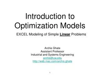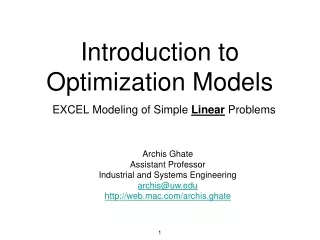
Optimization Models
Optimization Models. Module 9. OPTIMIZATION MODELS. EXTERNAL INPUTS. OUTPUT. MODEL. DECISION INPUTS. Optimization models answer the question, “What decision values give the best outputs?”. SCARCITY. DECISION INPUTS. CONSTRAINTS.


Optimization Models
E N D
Presentation Transcript
Optimization Models Module 9
OPTIMIZATION MODELS EXTERNAL INPUTS OUTPUT MODEL DECISION INPUTS Optimization models answer the question, “What decision values give the best outputs?”
SCARCITY DECISION INPUTS CONSTRAINTS Optimization models are necessary because resources are always limited.
LINEAR PROGRAMMING MODEL (objective function) 10x +18y DECISION INPUTS CONSTRAINTS OUTPUT 2x + 6y < 150 x x + .8y < 40 x + 1.5y < 50 y Linear programming is a special type of optimization model that sets up constraints as linear equations and solves them simultaneously while maximizing an objective function.
EXAMPLE 1: BOB’S MUFFLER SHOP Bob manufactures 2 types of mufflers, family and sport. Each family muffler nets him $10 and each sport muffler nets him $18. These numbers are known as the products’ ‘contribution margin’. His profit is determined by the function $10f + $18s, where f and s are the total number of each type of muffler sold. This is his objective function. His decision variables are the number of family and sport mufflers to manufacture each month. In an unconstrained situation, he would want to sell as many sport mufflers as because of their higher contribution. However…
EXAMPLE 1: BACKGROUND In order to create a muffler, Bob must use brackets, labor hours, and alloy. The resources needed for each type are: In any given month, he is limited in all three resources to these amounts: These are the problem constraints.
EXAMPLE 1: MODELING CONSTRAINTS AS LINEAR EQUATIONS These constraints can be modeled as a system of linear equations: 2f + 6s ≤ 150 (brackets) f + .8s ≤ 40 (labor) 50f + 33.33s ≤ 50 (alloy) Bob also has an outstanding contract that forces him to manufacture 5 sports style mufflers each month and knows, from historical performance, that demand for family mufflers in a given month will not exceed 35. These constraints can be modeled as: f ≤ 35 (maximum demand) s ≥ 5 (contractual obligation) The objective function (profit) is: 10f + 18s
This situation can be represented graphically. Consider the constraint imposed by brackets: 2f + 6s ≤ 150. If zero family mufflers are manufactured, the equation changes to (0)f + 6s ≤ 150, which reduces to s ≤ 25. Thus a maximum of 25 sports mufflers can be made if no family mufflers are made. Similarly, 75 family mufflers can be made if there are no sports mufflers manufactured. EXAMPLE 1: GRAPHING A CONSTRAINT Connecting these points gives a graphical representation of this constraint.
Points on the line are scenarios in which all available brackets are used. The area under the line is called the Range of Feasibility because it covers all product mixes that the constraint allows. Any point above the line is infeasible because Bob does not have enough brackets to create that combination of mufflers. EXAMPLE 1: RANGE OF FEASIBILITY Infeasible Point: (30 sport, 40 family) Range of Feasibility
The rest of the constraints can then be added in a similar fashion. EXAMPLE 1: GRAPHING ALL CONSTRAINTS 2f + 6s ≤ 150 (brackets) f + .8s ≤ 40 (labor) f + 1.5s ≤ 50 (alloy) f ≤ 35 (maximum demand) s ≥ 5 (contractual obligation)
The Range of Feasibility for the model is the area enclosed by all lines. EXAMPLE 1: THE COMPOSITE RANGE OF FEASIBILITY 2f + 6s ≤ 150 (brackets) f + .8s ≤ 40 (labor) f + 1.5s ≤ 50 (alloy) f ≤ 35 (maximum demand) s ≥ 5 (contractual obligation) Range of Feasibility
The profit function will be a line with the slope of -5/9, the ratio of the contribution margin of family mufflers to sports mufflers. Each line corresponds to a particular level of total profit. The further out the line is, the greater the amount of profit. EXAMPLE 1: POTENTIAL PROFIT LINES Total Profit: $100 $190 $280 $370 $460 $550
By combining the profit lines with the range of feasibility, you can identify the highest profit line that touches a feasible point. EXAMPLE 1: FEASIBLE PROFIT LINES
The optimal point is a mix of 25 family mufflers and 16.67 sport mufflers. This combination will net Bob $550. EXAMPLE 1: OPTIMAL SOLUTION VIA GRAPHICAL METHOD Optimal point
EXAMPLE 1: SPREADSHEET MODEL The situation can be modeled in Excel and an optimal solution found with Solver.
EXAMPLE 1: SPREADSHEET MODEL Contribution Margins Available resources Resources needed for each type of muffler Profit Max demand Contract Decisions: How many of each muffler to make Modeled constraints
EXAMPLE 1: SOLVER INPUTS Select the profit cell and choose solver from the tools menu.
Objective function (profit) EXAMPLE 1: SOLVER INPUTS Click Decision variables Constraints
EXAMPLE 1: SOLVER RESULTS Solver finds a solution. Select the answer and sensitivity reports for further analysis.
EXAMPLE 1: OPTIMAL SOLUTION Solver found the same optimal solution as the graphical method.
EXAMPLE 1: ANSWER REPORT ‘Binding’ means all available resources are used Brackets: 2f + 6s ≤ 150 Labor: f + .8s ≤ 40 The total resources used in the optimal solution Slack is the amount of leftover resources All available brackets are used in the optimal solution, making it a binding constraint. There are 1.67 labor hours left over, or slack.
EXAMPLE 1: SENSITIVITY ANALYSIS The allowable increase is the amount of resources that would have to be available to change the optimal solution. If 50 additional brackets are available, the optimal product mix will change. The allowable decrease is the amount of fewer resources that will change the optimal mix. The shadow price is the amount of profit that an additional unit of available resources would yield. A non-binding constraint will have a shadow price of 0 because there is already an excess of the resource. An additional available bracket (a total of 151) will yield $1 of profit. An additional labor hour will yield no profit because there is already an excess.
EXAMPLE 1: SENSITIVITY ANALYSIS The allowable increase and decrease tells you how sensitive the decision inputs of the optimal solution (final value column) are to the right hand sides of each constraint. If an additional unit of resource can be obtained for less than the shadow price, then the difference will be profit.
EXAMPLE 1: RANGE OF OPTIMALITY Profit: 10 f + 18 s The contribution margin for each type of muffler may be uncertain. The range of optimality is the range of contribution margins (coefficients in the objective function) in which a particular solution is the optimal solution.
EXAMPLE 1: RANGE OF OPTIMALITY Profit: 10 f + 18 s 8 ≤ contribution margin ≤ 14 15 ≤ contribution margin ≤ 30 Sports mufflers range: $18 + $12 = $30 $18 - $3 = $15 The range of optimality tells you how sensitive the decision inputs for the optimal solution are to variation in the coefficients of the objective function.