Download

1 / 33
330 likes | 506 Views
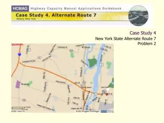
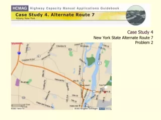
Case Study 4 New York State Alternate Route 7. Key Issues to Explore:. Capacity of the mainline sections of NYS-7 Adequacy of the weaving sections Performance of the interchange ramps Queuing Speed changes. After Working Through this Case Study You Should be able to:.

E N D
Key Issues to Explore: • Capacity of the mainline sections of NYS-7 • Adequacy of the weaving sections • Performance of the interchange ramps • Queuing • Speed changes
After Working Through this Case Study You Should be able to: • Determine the appropriate analyses required to address a similar problem. • Understand what input data are required and the assumptions that are commonly made. • Understand when and how to apply the methodologies. • Understand the limitations of the HCM procedures. • Reasonably interpret the results from an HCM analysis.
Observations? Network to be Studied I-87 / NY 7 Interchange NY 7: Basic Freeway Section I-787 / NY 7 Interchange
Problem 1: Basic Freeway Sections • 1a: Traffic Flow Patterns • Variation in volumes • Variations in the PHF • Speed-flow relationship • Flow-Occupancy • 1b: Basic Freeway Section Analysis (EB) • Selection of Appropriate Data • Basic Freeway Analysis • 1c: Analysis of WB Freeway Section • Number of Travel Lanes • Truck Climbing Lanes • Effect of Grades on Analyses
What time periods should be selected? What are the most important characteristics of this subarea? Do the defining characteristics differ by direction? How is the configuration of each basic freeway section likely to affect downstream system elements? AM PM AADT EB 3250 2400 29700 WB 2400 3500 30000 Observations? Peak Hour Volumes Length of basic freeway section = 3 miles
Determining traffic flow patterns using atypical conditions, where traffic data along the study roadway has been monitored for years. How many volume studies would need to be completed for the same degree of confidence? How else to account for the variability between data samples and typical roadway conditions? Observations? Sub-problem 1a
Observations? Flow Patterns AM Peak: 7-8 EB ~3500 vph WB ~ 2500 vph PM Peak: 4-5 EB ~2900 vph WB ~ 4000 vph Min flow between 2-3 am
Peak Hour Factor (PHF) • What is the relationship between hourly volumes and the peak hour factors? • When is there more variation in the PHF?
What is the typical mean speed? What happens as the flow increases? Observations? Speed Flow
Flow Occupancy • Is this what should be expected? • What volume should we select as being “typical” for the peak period analysis?
Observations? Trends in the Traffic Volume Which value is the right one to pick? Let’s say 90th percentile 95th Percentile = 3,385 vph 90th Percentile = 3,340 vph 50thPercentile = 3,096 vph Mean = 2,916 vph
Run Sub-problem 1b Perform basic freeway analysis of the eastbound section of Alternate Route 7.
Observations? Basic Freeway Section Analysis Methodology • What inputs are required? • Geometric Data • Free-flow Speed (FFS) • Volume Information
EB Segment Characteristics • The EB section has 2 lanes & is divided into 3 segments: • a one-mile segment with a 1-2% upgrade to the vicinity of Miller Road • a one-mile segment with a 1-2% downgrade • a final one-mile segment with a 5-7% downgrade ending at the I-787 interchange. Which segment should be chosen to do the analysis? The HCM says: use the section that will produce the most conservative estimate of the LOS. That is, worst case governs.
Obtaining the Free-Flow Speed • FFS can be obtained from: • Field measurements • Estimate from Chapter 23 of HCM
From Sub-problem 1a we have: Observations? Obtaining FFS using Field Data What is a good choice for the FFS? say ~55 MPH
Obtaining FFS Chapter 23 of HCM • The basic free flow speed (BFFS) is how fast vehicles are traveling when the volumes are light. • The HCM assumes the BFFS is 70 / 75 mph in urban / rural settings. (Field data shows that these values are too high) • The HCM allows us to use a local value rather than the defaults. Therefore use BFFS = 60 mph. • After using the HCM method in Chapter 23 what is the FFS? 55.5 MPH
Free Flow Speed • FFS from Field Observations = 55 MPH • FFS from HCM Chapter 23 = 55.5 MPH • Conclusion: Both methods provide similar results
V = 3,340 veh/hr (HCM Eqn 23-2) PHF = 0.90 N = 2 PT = 0.05 (field observations) PR = 0 (field observations) ET = 1.5 ER = 1.2 fp = 1.0 What is the average 15-minute passenger-car equivalent flow rate? vp = 1,902 passenger cars / hour / lane What additional data is needed to compute the LOS of this segment? Use the HCM to compute the average passenger car speed Additional Data
HCM Equations for Speed-Flow Relationship • If (55 ≤ FFS ≤ 75 mph) & (vp ≤ 3,400 – 30*FFS), then (from HCM Exhibit 23-3) S = FFS • If (55 ≤ FFS ≤ 70 mph) & (3,400 – 30*FFS <vp≤ 1,700 + 10*FFS), then (from HCM Exhibit 23-3) • And if (70 < FFS ≤ 75 mph) & (3,400 – 30*FFS) < vp ≤ 2,400, then (from HCM Exhibit 23-3) Then what does S equal? S = 54.8 MPH
LOS defined by the HCM for passenger cars /mile/lane: A: 0-11 B: 11-18 C: 18-26 D: 26-35 E: 35-45 Above 45 is LOS F Calculating the average density: D = vp / S D = 1,902 pcphpl / 54.8 mph D = 34.7 pcpmpl What does this mean using the 90th percentile to evaluate? - 10% of the time in the peak hour the EB LOS is D or worse - 90% of the time it is better than D during the peak hour Observations? Level of Service
What is the performance of this facility like during a reasonably heavy AM peak hour? Do these match the field observations? Range between the bars = LOS D (~80%) Mainly LOS D Yes, field data matches!!!
Perform basic freeway analysis of the westbound section of Alternate Route 7. This sub-problem is similar to 1b. Think about why conditions on the westbound section would be different than those on the eastbound section? Consider roadway users, physical conditions, and heavy vehicle needs. Observations? Sub-problem 1c
WB Segment Characteristics The WB section has 3 lanes and is divided into 3 segments: • 6-7% upgrade • 1-2% upgrade • 1-2% downgrade Which segment should be chosen to do the analysis? The HCM says: use the section that will produce the most conservative estimate of the LOS. That is, worst case governs.
V = 3,240 veh/hr PHF = 0.90 N = 3 FFS = 55 MPH (calculated similar to sub-problem 1b) PT = 0.05 (field observations) PR = 0 (field observations) ET = 1.5 ER = 1.2 fp = 1.0 What is the average 15-minute passenger-car equivalent flow rate? vp = 1,440 passenger cars / hour / lane What is the average passenger car speed? S = 55 MPH Additional Data
LOS defined by the HCM for passenger cars per mile per lane (pcpmpl): A: 0-11 B: 11-18 C: 18-26 D: 26-35 E: 35-45 Above 45 is LOS F Calculating the average density: D = vp / S D = 1,440 pcphpl / 55.0 mph D = 26 pcpmpl LOS = D Observations? Level of Service
Is the 3rd Lane Needed? • How would the system perform if only 2 lanes were available? • Vp = 2,160 pcphpl • D = 42 pcpmpl • S = 52 MPH • LOS = E The 3rd lane has a huge impact!!!
Truck Climbing Lane • What is the effect of the climbing lane? 5% trucks = 162 trucks/hr From HCM Exhibit 23-9: 162 trucks/hr = 810 passenger cars/hr What does this mean? ~ ½ lane worth of passenger car capacity is devoted to the trucks
Truck Lane: V=810 pcph * 2 = 1,620 pcph D=16.4 pcpmpl LOS = B Good Other 2 Lanes (no trucks): vp = 1,711 pcphpl, D= 31.1 pcpmpl, & LOS = D If all lanes used by all the traffic: D= 26.2 pcpmpl If trucks separated into climbing lane: Dtruck = 26.2 pcpmpl Dpass = 31.1 pcpmpl What does this mean? Enforcing a truck only lane is not a good idea!!! Observations? Should it be enforced that trucks can only use the climbing lane?
What if the truck percentage increased to 10%? ET would drop from 5 to 3.5 Why? When there are more trucks they begin to fill in the voids other trucks create The density would increase to 27.3 pcpmpl Questions
What is the predominate LOS for the peak hour? Is this reasonable? Observations? LOS for the 256 peak hours of the year (weekdays only) LOS = C
Observations? Level of Service • What effect would “regular drivers” vs. “vacationers” have on the system? • How likely are these situations? Regular drivers mainly provide a LOS = C and Vacationers mainly provide a LOS = D. Neither exactly describes the facility, probably somewhere in between