Understanding Coordinate Systems and Viewports in Computer Graphics
This document explores the fundamental concepts of coordinate systems in computer graphics, focusing on the essential pixel-based coordinates used in screen windows. It delves into the mapping of world coordinates to screen viewports and discusses how to define rectangular world windows and viewports. The content also covers the principles of mapping, clipping, and the impact of distortion when transitioning between different coordinate systems. Practical examples, including OpenGL functions for setting up viewports and world windows, are provided to illustrate these concepts.

Understanding Coordinate Systems and Viewports in Computer Graphics
E N D
Presentation Transcript
Computer Graphics Lab. Fall 2011 Hyunki Hong Dept. of Imaging Science & Arts, GSAIM Chung-Ang Univ.
Ch.3 More Drawing Tools 3.1 Introduction · the basic coordinate system of the screen window - coordinates that are essentially in pixels, - extending from zero to screenWidth-1 in x - from zero to some value screenHeight-1 in y. - use only positive values of x & y Ch.3 More Drawing Tools 3.1 Introduction · the basic coordinate system of the screen window - coordinates that are essentially in pixels, - extending from zero to screenWidth-1 in x - from zero to some value screenHeight-1 in y. - use only positive values of x & y · world coordinate - the space in which objects are described - the usual Cartesian xy-coordinates used in mathematics · define a rectangular world window in world coordinates → which part of the “world” should be drawn · define a rectangular viewport in the screen window
· A mapping between the world window & the viewport is established. → When all the objects in the world are drawn, the parts that lie inside the world window are automatically mapped to the inside of the viewport. : mapping + clipping · A mapping between the world window & the viewport is established. → When all the objects in the world are drawn, the parts that lie inside the world window are automatically mapped to the inside of the viewport. : mapping + clipping 3.2 World Windows & Viewports · Fig. 3.2 A plot of the “sinc” function : how the various (x, y) values become scaled & shifted so that the picture appears properly in the screen window. void myDisplay (void) { glBegin(GL_LINE_STRIP); for (Glfloat x = -4.0; x < 4.0; x += 0.1) { Glfloat y = sin(3.141592*x)/(3.141592*x); glVertex2f(x, y); } glEnd(); glFlush(); }
· Fig. 3.4 : a world window & a viewport - 3D "worlds" viewed with a "camera" 3.2.1 The mapping from the window to the viewport · Fig. 3.5 : Specifying the window & viewport
· Fig. 3.6: A picture mapped from a window to a viewport. → distortion occurs because the figure in the window must be stretched to fit into the viewport. · Fig. 3.6: A picture mapped from a window to a viewport. → distortion occurs because the figure in the window must be stretched to fit into the viewport. · window-to-viewport mapping - based on a formula that produces a point (sx, sy) in the screen window coordinates for any given point (x, y) in the world - Proportionality forces the mappings to have the linear form for some constants. : Eq. 3.2 & 3 (scale & shift constants) ex. aspect ratio
- in OpenGL a. gluOrtho2D( ): set the world window for 2D drawing void gluOrtho2D(GLdouble left, GLdouble right, GLdouble bottom, GLdouble top); b. glViewport( ): set the viewport void glViewport(GLint x, GLint y, GLint width, GLint height); · Ex. 3.2.4 & Fig. 3.10/11 - tiling the window : laying lots of copies of the same thing side by side to cover the entire screen window - motif : the picture that is copied at different positions 프로그램 확인 6/37
· Ex. 3.2.5 Clipping parts of a figure - zooming in & out: making the window smaller & larger - roaming (panning): shifting the window to a new position · Ex. 3.2.6 Zooming in on a figure in an animation cf. frames: a series of pictures - achieving a smooth animation a. a steady display of the current figure b. instantaneous replacement of the current figure by the new figure. 1) glutInitDisplayMode (GLUT_DOUBLE | GLUT_RGB) 2) double buffering : glutSwapBuffers() image in buffer → screen window · Fig. 3.14/15 (b) a tiling formed using many viewports 프로그램 예시 프로그램 연습
· Setting the window & viewport automatically - Setting of the window a. find a window that includes the entire object b. The extent (or bounding box) of an object is the aligned rectangular that just covers the object. c. How can be the extent be computed for a given object? 1) If all the endpoints of the object's lines are stored in an array : find the extreme values of the x- & y-coordinates in this array
2) If an object is procedurally defined, a) Execute the drawing routine, but do no actual drawing ; just compute the extent. Then set the window. b) Execute the drawing routine again. Do the actual drawing. d. Automatic setting of the viewport to preserve the aspect ratio e. Possible aspect ratios for the world and screen windows cf. anamorphic : 해상도 변환 고려 (16:9 → 4:3)
#include <windows.h> #include <gl/glut.h> void RenderScene(void) { // Clear the window with current clearing color glClear(GL_COLOR_BUFFER_BIT); // Set current drawing color to red : R G B glColor3f(1.0f, 0.0f, 0.0f); // Draw a filled rectangle with current color glRectf(100.0f, 150.0f, 150.0f, 100.0f); // Flush drawing commands glFlush(); } void SetupRC(void)// Setup the rendering state { glClearColor(0.0f, 0.0f, 1.0f, 1.0f);// Set clear color to blue } // Called by GLUT library when the window has chanaged size void ChangeSize(GLsizei w, GLsizei h) { // Prevent a divide by zero if(h == 0)h = 1; // Set Viewport to window dimensions glViewport(0, 0, w, h); 드로잉 연산 수행시 사용될 색 설정 void glRectf(GLfloat x1, GLfloat y1, GLfloat x2, GLfloat y2); x1 x2 윈도우 크기 변할 때마다 새로운 w, h를 인자로 받음. (automatic setting of the viewport to preserve the aspect ratio) void glViewport(GLint x, GLint y, GLsizei width, GLsizei height); 윈도우 내 일정영역을 스크린 좌표로 지정
// Reset coordinate system glMatrixMode(GL_PROJECTION); glLoadIdentity(); // Establish clipping volume (left, right, bottom, top, near, far) if (w <= h) glOrtho (0.0f, 250.0f, 0.0f, 250.0f*h/w, 1.0, -1.0); else glOrtho (0.0f, 250.0f*w/h, 0.0f, 250.0f, 1.0, -1.0); // glOrtho (0.0f, 250.0f, 0.0f, 250.0f, 1.0, -1.0); glMatrixMode(GL_MODELVIEW); glLoadIdentity(); } void main(void) { glutInitDisplayMode(GLUT_SINGLE | GLUT_RGB); glutCreateWindow("GLRect"); glutDisplayFunc(RenderScene); glutReshapeFunc(ChangeSize); SetupRC(); glutMainLoop(); } 행렬변환 수행되기 전에 좌표계 재설정(reset) = 현재변환행렬이 단위행렬로 설정 클리핑 공간의 범위 설정/수정 : 종횡비를 정사각형으로 유지 void glOrtho(GLdouble left, GLdouble right, GLdouble bottom, GLdouble top, Gldouble near, Gldouble far ); 현재 행렬 설정 GL_MODELVIEW: 행렬연산이 modelview 스택에 적용 장면 상에서 물체 이동시 GL_PROJECTION: projection 스택에 적용 클리핑 공간 정의시 GL_TEXTURE: texture 스택에 적용. 텍스쳐 좌표 설정시 윈도우 크기가 변할 때마다 ChangeSize 함수 호출
· Resizing the screen window; the resize event - In a window-based system the user can resize the screen window at run time, typically by dragging one of its corners with the mouse. → a resize event glutReshapeFunc(myReshape); //specifies the function called on a resize event void myReshape(GLsizei W, GLsizei H); // the system automatically passes the new width & height of the screen window · Making a matched viewport : find a new viewport that both fits into the new screen window and has the same aspect ratio as the world window ex. Using a reshape function to set the largest matching viewport upon a resize event. 3.3 Clipping Lines · keep those parts of an object that lie outside a given region from being drawn
3.3.1 How to clip a line · The Cohen-Sutherland clipper - compute which part (if any) of a line segment with endpoints lies inside the world window, - and then reports back the endpoints of that point. - clipSegment(p1, p2, window) - Fig. 3.16 : Clipping lines at window boundaries. a. If the entire line lies within the window (ex. CD) → 1 b. If the entire line lies outside the window (ex. AB) → 0 c. ED & AE → 1
3.3.2 The Cohen-Sutherland clipping algorithm : quickly detects and dispenses with two common cases, "trivial accept" & "trivial reject" · Fig. 3.17 - segment AB lie within window W → trivially accepted: no clipping - segment CD must lie entirely W → trivially rejected
· Testing for a Trivial Accept or Trivial Reject - an "inside-outside code word" is computed for each endpoint of the segment. : Fig. 3.18, 19 - form a code word for each of the endpoints of the line segment being tested a. trivial accept: Both code words are FFFF. b. trivial reject: The code words have a T in the same position. · Clipping when there is neither trivial accept nor trivial reject - If the segment can be neither trivially accepted nor rejected, it is broken into two parts at one of the window boundaries.
- Fig. 3.20 : Clipping a segment against an edge - Fig. 3.22 : A segment that requires four clips
cf. Developing the Canvas Class · canvas: A class provides a handy drawing canvas on which to draw the lines, polygons, etc. of interest. · Some useful supporting classes - class Points: a point having real coordinates → a single point expressed with floating-point coordinates - class IntRect: an aligned rectangle with integer coordinates → To describe a viewpoint, we need an aligned rectangle having integer coordinates. - class RealRect: an aligned rectangle with real coordinates → A world window requires the use of an aligned rectangle having real values for its boundary position. · Declaration of class canvas - The header file Canvas.h → include the current position, a window, a viewport, and the window-to-viewport mapping
- Implementation of some Canvas member functions · Relative Drawing - have drawing take place at the current position (CP) and to describe positions relative to the CP → changes in position - Developing moveRel( ) & lineRel( ) - Turtle graphics : It keeps track not only of "where we are" with the CP, but also "the direction in which we are headed (the current direction)."
a. The turtle is positioned at the CP, headed in a certain direction called the current direction, CD, the number of degrees measured counterclockwise (CCW) from the positive x-axis. b. add functionality to the Canvas class 1) turnTo (float angle) // CD=angle; 2) turn (float angle) // CD+=angle; 3) forward (float dist, int isVisible) 프로그램 확인 void Canvas:: forward(float dist, int isVisible) { const float RadPerDeg = 0.017453393; //radians per degree float x = CP.x + dist * cos(RadPerDeg * CD); float y = CP.y + dist * sin(RadPseDeg * CD); if(isVisible) lineTo(x, y); else moveTo(x, y); } 19/37
3.4 Regular Polygons, Circles, and Arcs 3.4.1 The regular polygons · A polygon is regular if it is simple, if all its sides have equal lengths, and if adjacent sides meet at equal interior angles. · n-gon : a regular polygon having n sides (Fig. 3.23) · the vertices of an n-gon lie on a circle : the parent circle of the n-gon · Finding the vertices of a 6-gon. 프로그램 확인 20/37
3.4.2 Variations on n-gons • · Fig 3.25 : The 7-gon and its offspring (stellation, 7-rosette) • · Ex. 3.4.1 The rosette and the golden 5-rosette • 3.4.3 Drawing Circles & Arcs • · Drawing a circle is equivalent to drawing • an n-gon that has a large number of vertices. • · Defining an arc • : described by the position of the center c & • radius R of its "parent" circle, along with • its beginning angle a & the angle b through which it sweeps in a CCW • direction from a 프로그램 확인
- a circle: an arc with a sweep of 360 degree · how to build a circle: a center & radius 3.4.4 Successive refinement of curves · Very complex curves can be fashioned recursively by repeatedly "refining" a simple curve. · Koch curve (by Helge von Koch, 1904) → an infinitely long line within a region of finite area - the zeroth-generation shape (K0): a horizontal line of length unity - To create K1, divide the line K0 into three equal parts. - and replace the middle section with a triangular "bump" having sides of length 1/3. → the total length of the line: 4/3. two generations of the Koch curve.
- To form Kn+1 from Kn: Subdivide each segment of Kn into three equal parts, and replace the middle part with a bump in the shape of an equilateral triangle. - Each segment is increased in length by a factor of 4/3. : Ki has total length (4/3)i, which increases as i increases. a. The first few generations of the Koch snowflake : 3(4/3)i. b. Koch snowflake, s3, s4, and s5.
cf. fractional dimension - In the limit, the Koch curve has infinite length, yet occupies a finite region in the plane. - An object has dimension D if, when it is subdivided into N equal parts, each part must be made smaller on each side by r = 1/N1/D. a. Taking logarithms on both sides of this equation: D = log(N) / log(1/r). ex. Koch curve: N = 4 segments are created from each parent segment, but their lengths are r = 1/3 → D = 1.26 b. If curve A has a larger value of D than curve B does, curve A is fundamentally more "wiggly" than B; that is, it is less "linelike" and more "plane filling."
cf. L-System: draw complex curves based on a simple set of rules - The turtle a. ‘F’ : forward(1,1) → go forward visibly a distance 1 in the CD. b. ‘+’ : turn (A) → turn right through angle A degrees. c. ‘-’ : turn(-A) → turn left through angle A degrees. - a set of string-production rules for the Koch curve : ‘F’ → “F-F++F-F” with angle (60°) - Fig. two stages of the string-production process a. In the first stage, an initial string called the atom, ("F") b. "produces" the first-generation string, (S1 = "F-F++F-F") - an Iterated Function System (IFS)
- Fractal trees a. the atom ‘F’, an angle of 22° b. the F-string: F → “FF – [-F + F + F] + [+F – F – F]” A fourth-orders “bush” First two orders of a bush Adding randomness & tapering to trees
3.5 The Parametric Form for a Curve · two ways to describe the shape of a curved line : implicitly & parametrically · the implicit form: a curve described by a function F(x, y) that provides a relationship between the x & y coordinates. - The point (x, y) lies on the curve if and only if it satisfies the equation: F(x, y) = 0. ex. x2 + y2 = r2 - a benefit: easily to test whether a given point lies on the line or curve - the inside-outside function: F(x, y) = x2 + y2 - R2 3.5.1 Parametric forms for curves → a wide variety of curves · the movement of a point through time → the motion of a pen as it sweeps out the curve cf. a explicit form cf. F(x, y) = 0 for all (x, y) on the curve …
· the path of a particule traveling along the curve is fixed by two functions x() & y() (x(t), y(t)) : the position of the particle at time t · Examples : the line (Eq. 3.11) & the ellipse (Eq. 3.12) · Fig. 3.39 : an ellipse described parametrically · Finding an implicit form from parametric form : combine the two equation for x(t) and y(t) to somehow eliminate the variable t. ex. Ellipse :
· conic section - ellipse : The plane cuts one nappe of the cone. - parabola : The plane is parallel to the side of the cone. → Implicit form : - hyperbola : The plane cuts both nappes of the cone. → Implicit form : · Fig. 3.40 The classical conic sections
- the general second-degree equation: - standard equation of an ellipse:
· 직선 vs. 곡선 → 직선과 곡선의 수학적 정의, 모델에 사용될 때의 행동 방식, 그들에 의한 3D 구조의 유형, 시각적 외관에서 각각 차이 존재. · 직선 - 두 점 사이의 최단 거리, - 폴리곤/폴리곤 메쉬를 만드는 데 사용되므로 poligonal line라고도 함. · 곡선 - 변화의 세밀한 구별이나 디자인의 우아함에 관계함. - 일반적으로 몇 개의 점에 의해 정의, 선분(curve segment)라고도 함. - 곡면 정의, 곡면의 메쉬 생성 가능 - spline (그림 : spline 수정을 위한 대표적인 조절 방식)
·Bézier curve(르노 자동차, 1971) The Bézier curve based on four points.
cf. Bezier curves don’t offer enough local control over the shape of the curve. → The set of blending functions give some local control to the control points. Example of a spline function : g(t)consists of three polynomial segments, defined as a(t) = ½t2 b(t) = ¾ - ( t – 3/2)2 c(t) = ½ (3 – t)2 The support of g(t)is [0 , 3]; a(1) = b(1) = ½ and b(2) = c(2) = ½ a´(1) = b´(1) = 1 and b´(2) = c´(2) = -1 Span : [0, 1], joint (t = 1, 2), Knots : the value of t piecewise polynomials
· The shape g(t) - an example of a spline function - a piecewise polynomial function that possesses “enough” smoothness · A spline curve : In an adjacent span, the curve is given by a different sum of polynomials, but we know that all segments meet to make the curve continuous. · B-spline : one basis in particular whose blending functions have the smallest support and therefore offer the greatest local control. · The rational polynomial functions → how the definition of a few points can determine the shape of a curve. P0, P1, P2 – control points.
a. The curve is one of the conic sections, and the type depends on the value of w: if w < 1, an ellipse. if w = 1, a parabola. if w > 1, a hyperbola. b. A rational spline curve is formed as the familiar blending of control points. shape parameter : a set of weight {w0, …. wL} Rk(t) : a ratio of polynomials (rational B-splines) c. The knot vector used to define the B-spline functions is usually nonuniform (not equispaced) → nonuniform rational B-splines (NURBS)
3.5.2 Drawing curves represented parametrically · It's straightforward to draw a curve when its parametric representation is available. · a curve C has the parametric representation P(t) = (x(t), y(t)) form as t varies from 0 to T. - Fig. 3.41 : Approximating curve by a polyline → samples of P(t) at closely spaced instants - Fig. 3.42 : Drawing a curve using points in t.
3.5.3 Polar coordinate shapes · Each point on the curve is represented by an angle θ and a radial distance r. · Fig. 3.44 & Eq. 3.18 : Polar coordinates · the logarithmic spiral: the only spiral that has the same shape for any change of scale cf. 3D curves - the curve is at P(t) = (x(t), y(t), z(t)) at time t. - the helix
Assignments (OpenGL Programming) : A “7-gram”, Rotating “pentathings”, The yin-yang symbol, The seven circles, The teardrop and its construction, Some figures based on the teardrop