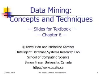
Data Mining: Concepts and Techniques

1. Data Mining: Concepts and Techniques These slides have been adapted from Han, J., Kamber, M., & Pei, Y. Data Mining: Concepts and Technique. Data Mining: Concepts and Techniques

2. Chapter 4: Data Cube Technology • Efficient Computation of Data Cubes • Exploration and Discovery in Multidimensional Databases • Summary Data Mining: Concepts and Techniques

3. Efficient Computation of Data Cubes • General heuristics • Multi-way array aggregation • BUC • H-cubing • Star-Cubing • High-Dimensional OLAP Data Mining: Concepts and Techniques

4. all 0-D(apex) cuboid time item location supplier 1-D cuboids time,location item,location location,supplier 2-D cuboids time,supplier item,supplier time,location,supplier 3-D cuboids item,location,supplier time,item,supplier 4-D(base) cuboid Cube: A Lattice of Cuboids time,item time,item,location time, item, location, supplier Data Mining: Concepts and Techniques

5. Preliminary Tricks • Sorting, hashing, and grouping operations are applied to the dimension attributes in order to reorder and cluster related tuples • Aggregates may be computed from previously computed aggregates, rather than from the base fact table • Smallest-child: computing a cuboid from the smallest, previously computed cuboid • Cache-results: caching results of a cuboid from which other cuboids are computed to reduce disk I/Os • Amortize-scans: computing as many as possible cuboids at the same time to amortize disk reads • Share-sorts: sharing sorting costs cross multiple cuboids when sort-based method is used • Share-partitions: sharing the partitioning cost across multiple cuboids when hash-based algorithms are used Data Mining: Concepts and Techniques

6. Efficient Computation of Data Cubes • General heuristics • Multi-way array aggregation • BUC • H-cubing • Star-Cubing • High-Dimensional OLAP Data Mining: Concepts and Techniques

7. Multi-Way Array Aggregation • Array-based “bottom-up” algorithm • Using multi-dimensional chunks • No direct tuple comparisons • Simultaneous aggregation on multiple dimensions • Intermediate aggregate values are re-used for computing ancestor cuboids • Cannot do Apriori pruning: No iceberg optimization Data Mining: Concepts and Techniques

8. C c3 61 62 63 64 c2 45 46 47 48 c1 29 30 31 32 c 0 B 60 13 14 15 16 b3 44 28 56 9 b2 B 40 24 52 5 b1 36 20 1 2 3 4 b0 a0 a1 a2 a3 A Multi-way Array Aggregation for Cube Computation (MOLAP) • Partition arrays into chunks (a small subcube which fits in memory). • Compressed sparse array addressing: (chunk_id, offset) • Compute aggregates in “multiway” by visiting cube cells in the order which minimizes the # of times to visit each cell, and reduces memory access and storage cost. What is the best traversing order to do multi-way aggregation? Data Mining: Concepts and Techniques

9. C c3 61 62 63 64 c2 45 46 47 48 c1 29 30 31 32 c 0 B 60 13 14 15 16 b3 44 28 56 9 b2 40 24 52 5 b1 36 20 1 2 3 4 b0 a0 a1 a2 a3 A Multi-way Array Aggregation for Cube Computation B Data Mining: Concepts and Techniques

10. Multi-way Array Aggregation for Cube Computation C c3 61 62 63 64 c2 45 46 47 48 c1 29 30 31 32 c 0 B 60 13 14 15 16 b3 44 28 B 56 9 b2 40 24 52 5 b1 36 20 1 2 3 4 b0 a0 a1 a2 a3 A Data Mining: Concepts and Techniques

11. Multi-Way Array Aggregation for Cube Computation (Cont.) • Method: the planes should be sorted and computed according to their size in ascending order • Idea: keep the smallest plane in the main memory, fetch and compute only one chunk at a time for the largest plane • Limitation of the method: computing well only for a small number of dimensions • If there are a large number of dimensions, “top-down” computation and iceberg cube computation methods can be explored Data Mining: Concepts and Techniques

12. Efficient Computation of Data Cubes • General heuristics • Multi-way array aggregation • BUC • H-cubing • Star-Cubing • High-Dimensional OLAP Data Mining: Concepts and Techniques

13. Bottom-Up Computation (BUC) • BUC • Bottom-up cube computation (Note: top-down in our view!) • Divides dimensions into partitions and facilitates iceberg pruning • If a partition does not satisfy min_sup, its descendants can be pruned • If minsup = 1 Þ compute full CUBE! • No simultaneous aggregation Data Mining: Concepts and Techniques

14. BUC: Partitioning • Usually, entire data set can’t fit in main memory • Sort distinct values, partition into blocks that fit • Continue processing • Optimizations • Partitioning • External Sorting, Hashing, Counting Sort • Ordering dimensions to encourage pruning • Cardinality, Skew, Correlation • Collapsing duplicates • Can’t do holistic aggregates anymore! Data Mining: Concepts and Techniques

15. Efficient Computation of Data Cubes • General heuristics • Multi-way array aggregation • BUC • H-cubing • Star-Cubing • High-Dimensional OLAP Data Mining: Concepts and Techniques

16. H-Cubing: Using H-Tree Structure • Bottom-up computation • Exploring an H-tree structure • If the current computation of an H-tree cannot pass min_sup, do not proceed further (pruning) • No simultaneous aggregation Data Mining: Concepts and Techniques

17. Q.I. Q.I. Q.I. H-tree: A Prefix Hyper-tree root Header table bus hhd edu Jan Mar Jan Feb Tor Van Tor Mon Data Mining: Concepts and Techniques

18. Q.I. Q.I. Q.I. Computing Cells Involving “City” From (*, *, Tor) to (*, Jan, Tor) Header Table HTor root Bus. Hhd. Edu. Jan. Mar. Jan. Feb. Tor. Van. Tor. Mon. Data Mining: Concepts and Techniques

19. Q.I. Q.I. Q.I. Q.I. Computing Cells Involving Month But No City • Roll up quant-info • Compute cells involving month but no city root Hhd. Bus. Edu. Jan. Mar. Jan. Feb. Tor. Mont. Van. Tor. Top-k OK mark: if Q.I. in a child passes top-k avg threshold, so does its parents. No binning is needed! Data Mining: Concepts and Techniques

20. Q.I. Q.I. Q.I. Q.I. Computing Cells Involving Only Cust_grp root Check header table directly bus hhd edu Jan Mar Jan Feb Tor Van Tor Mon Data Mining: Concepts and Techniques

21. Efficient Computation of Data Cubes • General heuristics • Multi-way array aggregation • BUC • H-cubing • Star-Cubing • High-Dimensional OLAP Data Mining: Concepts and Techniques

22. Star-Cubing: An Integrating Method • D. Xin, J. Han, X. Li, B. W. Wah, Star-Cubing: Computing Iceberg Cubes by Top-Down and Bottom-Up Integration, VLDB'03 • Explore shared dimensions • E.g., dimension A is the shared dimension of ACD and AD • ABD/AB means cuboid ABD has shared dimensions AB • Allows for shared computations • e.g., cuboid AB is computed simultaneously as ABD • Aggregate in a top-down manner but with the bottom-up sub-layer underneath which will allow Apriori pruning • Shared dimensions grow in bottom-up fashion Data Mining: Concepts and Techniques

23. Iceberg Pruning in Shared Dimensions • Anti-monotonic property of shared dimensions • If the measure is anti-monotonic, and if the aggregate value on a shared dimension does not satisfy the iceberg condition, then all the cells extended from this shared dimension cannot satisfy the condition either • Intuition: if we can compute the shared dimensions before the actual cuboid, we can use them to do Apriori pruning • Problem: how to prune while still aggregate simultaneously on multiple dimensions? Data Mining: Concepts and Techniques

24. Cell Trees • Use a tree structure similar to H-tree to represent cuboids • Collapses common prefixes to save memory • Keep count at node • Traverse the tree to retrieve a particular tuple Data Mining: Concepts and Techniques

25. Star Attributes and Star Nodes • Intuition: If a single-dimensional aggregate on an attribute value p does not satisfy the iceberg condition, it is useless to distinguish them during the iceberg computation • E.g., b2, b3, b4, c1, c2, c4, d1, d2, d3 • Solution: Replace such attributes by a *. Such attributes are star attributes, and the corresponding nodes in the cell tree are star nodes Data Mining: Concepts and Techniques

26. Example: Star Reduction • Suppose minsup = 2 • Perform one-dimensional aggregation. Replace attribute values whose count < 2 with *. And collapse all *’s together • Resulting table has all such attributes replaced with the star-attribute • With regards to the iceberg computation, this new table is a loseless compression of the original table Data Mining: Concepts and Techniques

27. Star Tree • Given the new compressed table, it is possible to construct the corresponding cell tree—called star tree • Keep a star table at the side for easy lookup of star attributes • The star tree is a loseless compression of the original cell tree Data Mining: Concepts and Techniques

28. Star-Cubing Algorithm—DFS on Lattice Tree Data Mining: Concepts and Techniques

29. Multi-Way Aggregation Data Mining: Concepts and Techniques

30. Star-Cubing Algorithm—DFS on Star-Tree Data Mining: Concepts and Techniques

31. Multi-Way Star-Tree Aggregation • Start depth-first search at the root of the base star tree • At each new node in the DFS, create corresponding star tree that are descendents of the current tree according to the integrated traversal ordering • E.g., in the base tree, when DFS reaches a1, the ACD/A tree is created • When DFS reaches b*, the ABD/AD tree is created • The counts in the base tree are carried over to the new trees Data Mining: Concepts and Techniques

32. Multi-Way Aggregation (2) • When DFS reaches a leaf node (e.g., d*), start backtracking • On every backtracking branch, the count in the corresponding trees are output, the tree is destroyed, and the node in the base tree is destroyed • Example • When traversing from d* back to c*, the a1b*c*/a1b*c* tree is output and destroyed • When traversing from c* back to b*, the a1b*D/a1b* tree is output and destroyed • When at b*, jump to b1 and repeat similar process Data Mining: Concepts and Techniques

33. Efficient Computation of Data Cubes • General heuristics • Multi-way array aggregation • BUC • H-cubing • Star-Cubing • High-Dimensional OLAP Data Mining: Concepts and Techniques

34. The Curse of Dimensionality • None of the previous cubing method can handle high dimensionality! • A database of 600k tuples. Each dimension has cardinality of 100 and zipf of 2. Data Mining: Concepts and Techniques

35. Motivation of High-D OLAP • Challenge to current cubing methods: • The “curse of dimensionality’’ problem • Iceberg cube and compressed cubes: only delay the inevitable explosion • Full materialization: still significant overhead in accessing results on disk • High-D OLAP is needed in applications • Science and engineering analysis • Bio-data analysis: thousands of genes • Statistical surveys: hundreds of variables Data Mining: Concepts and Techniques

36. Fast High-D OLAP with Minimal Cubing • Observation: OLAP occurs only on a small subset of dimensions at a time • Semi-Online Computational Model • Partition the set of dimensions into shell fragments • Compute data cubes for each shell fragment while retaining inverted indices or value-list indices • Given the pre-computed fragment cubes, dynamically compute cube cells of the high-dimensional data cube online Data Mining: Concepts and Techniques

37. Properties of Proposed Method • Partitions the data vertically • Reduces high-dimensional cube into a set of lower dimensional cubes • Online re-construction of original high-dimensional space • Lossless reduction • Offers tradeoffs between the amount of pre-processing and the speed of online computation Data Mining: Concepts and Techniques

38. Example Computation • Let the cube aggregation function be count • Divide the 5 dimensions into 2 shell fragments: • (A, B, C) and (D, E) Data Mining: Concepts and Techniques

39. 1-D Inverted Indices • Build traditional invert index or RID list Data Mining: Concepts and Techniques

40. Generalize the 1-D inverted indices to multi-dimensional ones in the data cube sense Compute all cuboids for data cubes ABC and DE while retaining the inverted indices For example, shell fragment cube ABC contains 7 cuboids: A, B, C AB, AC, BC ABC This completes the offline computation stage Cell Intersection TID List List Size a1 b1 1 2 3 1 4 5 1 1 a1 b2 1 2 3 2 3 2 3 2 a2 b1 4 5 1 4 5 4 5 2 a2 b2 4 5 2 3 0 Shell Fragment Cubes: Ideas Data Mining: Concepts and Techniques

41. Shell Fragment Cubes: Size and Design • Given a database of T tuples, D dimensions, and F shell fragment size, the fragment cubes’ space requirement is: • For F < 5, the growth is sub-linear • Shell fragments do not have to be disjoint • Fragment groupings can be arbitrary to allow for maximum online performance • Known common combinations (e.g.,<city, state>) should be grouped together. • Shell fragment sizes can be adjusted for optimal balance between offline and online computation Data Mining: Concepts and Techniques

42. ID_Measure Table • If measures other than count are present, store in ID_measure table separate from the shell fragments Data Mining: Concepts and Techniques

43. The Frag-Shells Algorithm • Partition set of dimension (A1,…,An) into a set of k fragments (P1,…,Pk). • Scan base table once and do the following • insert <tid, measure> into ID_measure table. • for each attribute value ai of each dimension Ai • build inverted index entry <ai, tidlist> • For each fragment partition Pi • build local fragment cube Si by intersecting tid-lists in bottom- up fashion. Data Mining: Concepts and Techniques

44. Frag-Shells (2) Dimensions D Cuboid EF Cuboid DE Cuboid ABC Cube DEF Cube Data Mining: Concepts and Techniques

45. Online Query Computation: Query • A query has the general form • Each ai has 3 possible values • Instantiated value • Aggregate * function • Inquire ? function • For example, returns a 2-D data cube. Data Mining: Concepts and Techniques

46. Online Query Computation: Method • Given the fragment cubes, process a query as follows • Divide the query into fragment, same as the shell • Fetch the corresponding TID list for each fragment from the fragment cube • Intersect the TID lists from each fragment to construct instantiated base table • Compute the data cube using the base table with any cubing algorithm Data Mining: Concepts and Techniques

47. Online Query Computation: Sketch Instantiated Base Table Online Cube Data Mining: Concepts and Techniques

48. Experiment: Size vs. Dimensionality (50 and 100 cardinality) • (50-C): 106 tuples, 0 skew, 50 cardinality, fragment size 3. • (100-C): 106 tuples, 2 skew, 100 cardinality, fragment size 2. Data Mining: Concepts and Techniques

49. Experiment: Size vs. Shell-Fragment Size • (50-D): 106 tuples, 50 dimensions, 0 skew, 50 cardinality. • (100-D): 106 tuples, 100 dimensions, 2 skew, 25 cardinality. Data Mining: Concepts and Techniques

50. Experiment: Run-time vs. Shell-Fragment Size • 106tuples, 20 dimensions, 10 cardinality, skew 1, fragment size 3, 3 instantiated dimensions. Data Mining: Concepts and Techniques