Download
1 / 20
200 likes | 351 Views
Sensitivity . Professor Walter W. Olson Department of Mechanical, Industrial and Manufacturing Engineering University of Toledo. Outline of Today’s Lecture. Review Static Error Constants (Review) Loop Shaping Loop Shaping with the Bode Plot Lead and Lag Compensators

E N D
Sensitivity Professor Walter W. Olson Department of Mechanical, Industrial and Manufacturing Engineering University of Toledo
Outline of Today’s Lecture • Review • Static Error Constants (Review) • Loop Shaping • Loop Shaping with the Bode Plot • Lead and Lag Compensators • Lead design with Bode plot • Lead design with root locus • Lag design with Bode plot • Important transfer functions • Gang of Six • Gang of Four • Disturbance Rejection • Noise Rejection • Limitations
Static Error Constants • If the system is of type 0 at low frequencies will be level. • A type 0 system, (that is, a system without a pole at the origin,)will have a static position error, Kp, equal to • If the system is of type 1 (a single pole at the origin) it will have a slope of -20 dB/dec at low frequencies • A type 1 system will have a static velocity error, Kv, equal to the value of the -20 dB/dec line where it crosses 1 radian per second • If the system is of type 2 ( a double pole at the origin) it willhave a slope of -40 dB/dec at low frequencies • A type 2 system has a static acceleration error,Ka, equal to the value of the -40 dB/dec line where it crosses 1 radian per second
Loop Shaping Error signal E(s) • We have seen that the open loop transfer function, has profound influences on the closed loop response • The key concept in loop shaping designs is that there is some ideal open loop transfer (B(s)) that will provide the design specifications that we require of our closed loop system • Loop shaping is a trial and error process • To perform loop shaping we can used either the root locus plots or the Bode plots depending on the type of response that we wish to achieve • We have already considered an important form of loop shaping as the PID controller Output y(s) Input r(s) Controller C(s) Plant P(s) Open Loop Signal B(s) Sensor -1 + +
Loop Shaping with the Bode Plot • The open loop Bode plot is the natural design tool when designing in the frequency domain. • For the frequency domain, the common specifications are bandwidth, gain cross over frequency, gain margin, resonant frequency, resonant frequency gain, phase margin, static errors and high frequency roll off. -3 db Roll off Rate dB/dec Resonant peak gain, dB Bandwidth rps Resonant peak frequency rps Gain cross over frequency rps
Loop Shaping with the Bode Plot Increase of gain also increases bandwidth and resonant gain Break frequency corresponds to the component pole or zero Poles bend the magnitude and phase down Zeros bend the magnitude and the phase up
Lead and Lag Compensators • The compensator with a transfer functionis called a lead compensator if a<b and a lag compensator if a>b • The lead and the lag compensator can be used together • Note: the compensator does add a steady state gain ofthat needs to be accounted for in the final design • There are analytical methods for designing these compensators (See Ogata or Franklin and Powell)
Lead Compensator • The lead compensator is used to improve stability and to improve transient characteristics. • The lead compensator can be designed using either frequency response or root locus methods • Usually, the transient characteristics are better addressed using the root locus methods • Addressing excessive phase lag is better addressed using the frequency methods • The pole of the system is usually limited by physical limitations of the components use to implement the compensator • In the lead compensator, the zero and pole are usually separated in frequency from about .4 decades to 1.5 decades depending on the design
Lead Compensator (Frequency Design) Mechanical Lead Compensator Note: the lead compensator opensup the high frequency regionwhich could cause noise problems The Lead compensator addsphase b1 xi b2 x0 k y f wm
Lag Compensator • Lag compensators are used to improve steady state characteristics where the transient characteristics are adequate and to attenuate high frequency noise • In order to not change the transient characteristics, the zero and pole are located near the origin on the root locus plot • The starting point for the design on a root locus is to start with a pole location at about s = -0.001 and then locate the pole as needed for the desired effect • In order to not give up too much phase, the zero and pole are located away from the phase margin frequency
Lag Compensator Mechanical Lag Compensator xi b2 k a b b1 Note that the lag compensator causes a drop in the magnitude and phase This could be useful in reducing bandwidth, and improving gain margin; however it might reduce phase margin x0
Sensitivity • Sensitivity is an evaluation of how the system responds to various signals compared to the design signal • In general, we want the system to respond to the reference input • We do not want the system to respond to noises and other signals that do not contribute to the accuracy of the desired output
Several Transfer Functions N D Measurement Noise Disturbances u h Y U R E + + Y -1 Controller Process + + + +
The Model N D u h R Y U E + + Y -1 Controller Process “Gang of Six” Complementary Sensitivity Function Load Sensitivity Function + + + “Gang of Four” + Noise Sensitivity Function Sensitivity Function
Example N D u h Y U R E + + Y -1 Controller Process + + + +
Disturbance Rejection N D • We want our system designed such that the disturbances to the system are attenuated • Harold S. Black gave us the answer: negative feedback u h Y U R E + + Y -1 Controller Process + + + +
Disturbance Rejection Disturbances with a frequency less than the cross over frequency are attenuated while frequencies higher would be passed Fortunately, most load disturbances are low frequency and often can be treated as step inputs
Noise Rejection • We would also like noise rejection • Noise is most often high frequency signals caused by the sensors used to measure • Noise is presented as a result of the feedback terms • We do not have noise as defined here in an open system • In the closed loop error, noise is multiplied by T, the complementary sensitivity function, • In a system without a pre-filter, this is the transfer function • For this reason high frequency roll-off is important
Limitations • Systems with right hand side poles and zeros are inherently hard to control • For a system with right hand side poles, pk, Bode showed that • Improvements in one frequency region are met with deteriorations in another frequency region • Sometimes called the waterbed effect
Summary • Important transfer functions • Gang of Six • Gang of Four • Disturbance Rejection • Noise Rejection • Limitations Next: Robustness