Download
1 / 12
120 likes | 203 Views
Learn about Hidden Markov Models (HMM) in genetic data analysis, exploring the concept of semi-Markov chains, transition probabilities, and practical applications in experimental crosses. Discover how HMM helps analyze genetic inheritance patterns.

E N D
HMM in crosses and small pedigrees Lecture 8, Statistics 246, February 17, 2004
Discrete-time Markov chains • Consider a sequence of random variables X1,X2, X3, …with common finite state spaceS. This sequence forms a Markov chain if for all t, {X1 ,…,Xt-1} and {Xt+1 ,Xt+2 ,…} are conditionally independent given Xt , equivalently, • pr(Xt |Xt-1,Xt-2 ,…) = pr(Xt |Xt-1). • The matrix p(i,j;t) = pr(Xt = j |Xt-1 = i) is the transition matrix at step t. • When p(i,j;t) = p(i,j) for all i and j, independent of t, we say the Markov chain is time-homogeneous, or has stationary transition probabilities. Many of the chains we’ll be meeting will be inhomogeneous, and t will be in space, not time. • There are plenty of good books on elementary Markov chain theory, Feller vol 1 being my favourite, but they mostly concentrate on asymptotic behaviour in the homogeneous case. For the time being we don’t need this, or much else from the general theory, apart from the fact that multi-step transition matrices are products of 1-step transition matrices (Exercise).
Hidden Markov Models (HMM) • If (Xt) is a Markov chain, and f is an arbitrary function on the state space, then (f(Xt)) will not in general be a Markov chain. • Exercise: Construct an example to demonstrate the last assertion. • It is sometimes the case that associated with a Markov chain (Xt) is another process, (Yt) say, whose terms are conditionally independent given the chain(Xt). This happens with so-called semi-Markov chains. • Both functions of Markov chains and this last situation are covered by the following useful definition, based on the work of L. E. Baum and colleagues around 1970. A bivariate Markov chain (Xt,Yt) is called a Hidden Markov Model if a) (Xt) is a Markov chain, and b) the distribution of Ytgiven Xt , Xt-1 , Xt-2 …. depends only on Xt and Xt-1 . In many examples, this dependence is only on Xt , but in some, it can extendbeyond Xt-1 , and/or includeYt . Once you see how the defining property is used in the calculations, you will get an idea of the possible extensions. • Exercise. Explain how functions of Markov chains are always HMM.
HMM, cont. • There are many suitable references on HMM, but two good ones for our purposes are the books by Timo Koski (HMM for bioinformatics, 2001) and Durbin et al (Biological sequence analysis, 1998). • The simplest specification of an HMM is via the transition probabilitiesp(i,j;t) for the underlying Markov chain (Xt), and the emission probabilities for the observations (Yt), where these are given by • q(i,j, k;t) = pr(Yt = k | Xt-1 = i, Xt = j). • We also need an initial distribution for the chain: (i) = pr(X0 = i). • In general we are not going to observe (Xt ), which accounts for the word “hidden” in the name, but if we did, the probability of observing the state sequencex0 ,x1, x2, ….., xn, and associated observationsy1, y2, …,ynis • (x0)p(x0,x1;1)q(x0, x1 ,y1;1)…..p(xn-1,xn ;n )q(xn-1,xn,yn;n).
HMM in experimental crosses • We are going to consider the chromosomes of offspring from crosses of inbred strains A and B of mice. Suppose that we have n markers along a chromosome, #1 say, in their correct order 1, 2, …n, say, with rt being the recombination fraction between markers t and t+1. Consider the genotypes at these markers along chromosome 1 of an A H backcross mouse. Each genotype will be either A = aa or H = ab, and you can do the • Exercise. Under the assumption of no interference, the sequence of genotypes at markers 1, 2, …, n is a Markov chain with state space {A, H}, initial distribution (1/2,1/2 ), and 22 transition probability matrix R(rt) having diagonal entries1-rtfor no change (AA, HH), and off-diagonal entries rt for change (AH, HA). • This Markov chain represents the crossover process along the chromosome passed by one parent, say the mother. In an F2 intercross, H H, there is a crossover process in bothF1 parents. If we consider the offspring’s possible ordered genotypes, that is, genotypes with known parental origin (also called known phase), then the sequence of ordered genotypes at markers 1, 2, …, n is also a Markov chain, with state space, {a,b} {a,b} = {aa, ab, ba, bb}, initial distribution (1/2, 1/2) (1/2, 1/2) = (1/4,1/4, 1/4. 1/4), and transition probability matrixP(t) = R(rt)R(rt).
HMM in experimental crosses, cont • between marker t and t+1. Here you need to know the notion of tensor product of matrices, also known as direct product or Kronecker product. This is defined in most books on matrices, but my favourite is Bellman’s book • Exercise. My notation suggests the idea of the product of two independent Markov chains. Define this notion carefully, and show we get a Markov chain. • . • Now, unlike in the backcross, the observedF2 genotypes do not always tell us which parental strand had a recombination across an interval, and which didn’t, so we cannot always reconstruct the ordered genotypes. • With this 4-state Markov chain we have just 3 possible observed states, and we include some ambiguity states, giving us an observation space {A, H, B, C, D, -}, where C = {H,B} = not A, D = {A, H} = not B, and - = missing. • The resulting joint chain-observation process is an HMM, with emission probabilities which in a more general form can be written as the array on the next page. There is the error rate, which may in fact be marker specific, though for simplicity that is not indicated by the notation.
F2 HMM emission probabilities Note that the row entries in this array do not simply sum to 1, but the entries for mutually exclusive and exhaustive cases should: A, H and B, or A and C, etc.
Calculations with our HMM • For our F2 intercross there are certain calculations we would like to do which the HMM formalism makes straightforward. In fact, they are all instances of calculations generally of interest with HMM, and if the number of steps is not too large, and the state spaces not too big, there are neat algorithms for carrying them out which are worth knowing. • Major problems: Given the combined observations O of the genotypes Y = (Y1, Y2 ,…, Yn) from many different F2offspring, transition matrices P(rt), and emission probabilitiesq(t), t=1,2,…,n, • a) calculate the log likelihoodl( r | O) = log pr( O | r) for different parameter values and different marker orders; • b) calculate MLE for the recombination fractions r by maximizing l( r | O); • and for individual offspring with genotype dataY, • c) probabilistically reconstruct the individual unobserved ordered genotypesX = (X1, X2 ,….,,Xn ) by calculating argmaxX pr( X | Y, r). • We’ll see the algorithms in due course. We might also wish to simulate from pr( X | Y, r).
Another problem: reconstructing haplotypes The problem here is to reconstruct the childrens’ haplotypes as in the figure, from marker data on both the children and the parents.
Some basic notions from pedigree analysis • Founders: individuals without parents in the pedigree. • Non-founders: individuals with one or more parent in the pedigree • Calculations on pedigrees typically involve evaluating probabilities of data under specific hypotheses, perhaps going on to form likelihood ratios, or inferring unobserved genetic states, e.g. of genotypes or haplotypes. • To get started we need (in addition to the pedigree) phenotypic data, e.g. on markers or disease states, and a full genetic model. This means population genotype or allele frequencies, transmission probabilities, (probabilities of offspring haplotypes given parental haplotypes), and penetrances (probabilties of phenotypes given genotypes). Generally genotype frequencies in populations are assumed to satisfy the Hardy-Weinberg equlibrium formulae, and to be in linkage equilibrium across loci, and no interference is assumed in recombination. All of these are simplifications which have been found to be generally satisfactory.
Inheritance vectors • We plan to view our (small) pedigree as one large HMM. The states of the Markov chain along each chromosome are what we term inheritance vectors, which have a component for every meiosis in the pedigree, and entries 0 or 1. So if we have n non-founders, our inheritance vectors are binary vectors of length 2n. Each non-founder has 2 components of the inheritance vector assigned to them: one for their maternal and one for their paternal meiosis. At any locus on a chromosome, the entries in the inheritance vector for a non-founder are 0 if the parental variant passed on at that locus was grandmaternal, and 1 otherwise. For individuals whose parent are founders, this definition is incomplete, but we will make a choice below. Before doing so, let me note that slightly different definitions of inheritance vector are in the literature, and in Lange’s excellent book, they are replaced by what he terms descent graphs. Clearly the idea is the same: given an inheritance vector, and allelic assignments for the founders, we can follow the descent of the alleles down the pedigree using our vector, and it it is easy to envisage its graphical representation. • Consider a two-parent two-child nuclear family and suppose that the parents are 1/2 and 3/4, while the first child is 1/3 and the second is 2/4. Then the inheritance vector is of length 4, v = (vgm , vgp , vbm, vbp), where gm represents the girl’s maternal meiosis, gp her paternal meiosis, and so on.
Exercises and references • Exercise 1. Figure out whether the sequence of observed states (i.e. A, H, or B) in an F2 intercross is a Markov chain. (I asserted that collapsing the state space of a Markov chain will not, in general, lead to another Markov chain. But sometime it does. Does it in this case?) • Exercise 2. Suppose that 1, 2 and 3 are markers along a backcross mouse’s chromosome in that order, and that Xtdenotes its genotype at marker t. Prove that (contrary to my assertion in class) in general (X1,X2,X3) will notbe Markov in the incorrect order, e.g. that in general, • pr(X2 = H | X1 = A, X3 = H) pr (X2 = H | X1 = A), • which would be true if (X3,X1,X2) were Markov in that order (3-1-2). • References. As already mentioned, Lange’s book is a good reference for this topic applied to genetics. Closely related material can be found in my old class notes on my web site, see my Stat 260 for 1998, esp. weeks 3, 7 and 8, and weeks 3, 6 and 7 of 2000.