Download
1 / 175
1.77k likes | 2.22k Views
Learn key concepts of probability theory and stochastic processes, including random variables, distributions, functions, and transformations. Covering various distributions like Poisson, Exponential, and Normal. Understand Stochastic Processes like Poisson process and Markov chains.

E N D
Probability and Stochastic Processes References: Wolff, Stochastic Modeling and the Theory of Queues, Chapter 1 Altiok, Performance Analysis of Manufacturing Systems, Chapter 2 Chapter 0
Basic Probability • Envision an experiment for which the result is unknown. The collection of all possible outcomes is called the sample space. A set of outcomes, or subset of the sample space, is called an event. • A probability space is a three-tuple (W ,, Pr) where W is a sample space, is a collection of events from the sample space and Pr is a probability law that assigns a number to each event in . For any events A and B, Pr must satsify: • Pr() = 1 • Pr(A) 0 • Pr(AC) = 1 – Pr(A) • Pr(A B) = Pr(A) + Pr(B), if A B = . • If A and B are events in with Pr(B) 0, the conditional probability of A given B is Chapter 0
Random Variables A random variable is “a number that you don’t know… yet” Sam Savage, Stanford University • Discrete vs. Continuous • Cumulative distribution function • Density function • Probability distribution (mass) function • Joint distributions • Conditional distributions • Functions of random variables • Moments of random variables • Transforms and generating functions Chapter 0
Functions of Random Variables • Often we’re interested in some combination of r.v.’s • Sum of the first k interarrival times = time of the kth arrival • Minimum of service times for parallel servers = time until next departure • If X = min(Y, Z) then • therefore, • and if Y and Z are independent, • If X = max(Y, Z) then • If X = Y + Z , its distribution is the convolution of the distributions of Y and Z. Find it by conditioning. Chapter 0
Conditioning (Wolff) • Frequently, the conditional distribution of Y given X is easier to find than the distribution of Y alone. If so, evaluate probabilities about Y using the conditional distribution along with the marginal distribution of X: • Example: Draw 2 balls simultaneously from urn containing four balls numbered 1, 2, 3 and 4. X = number on the first ball, Y = number on the second ball, Z = XY. What is Pr(Z > 5)? • Key: Maybe easier to evaluate Z if X is known Chapter 0
Convolution • Let X = Y+Z. • If Y and Z are independent, • Example: Poisson • Note: above is cdf. To get density, differentiate: Chapter 0
Moments of Random Variables • Expectation = “average” • Variance = “volatility” • Standard Deviation • Coefficient of Variation Chapter 0
Linear Functions of Random Variables • Covariance • Correlation If X and Y are independent then Chapter 0
Transforms and Generating Functions • Moment-generating function • Laplace transform (nonneg. r.v.) • Generating function (z – transform) Let N be a nonnegative integer random variable; Chapter 0
Special Distributions • Discrete • Bernoulli • Binomial • Geometric • Poisson • Continuous • Uniform • Exponential • Gamma • Normal Chapter 0
Bernoulli Distribution “Single coin flip” p = Pr(success) N = 1 if success, 0 otherwise Chapter 0
Binomial Distribution “n independent coin flips” p = Pr(success) N = # of successes Chapter 0
Geometric Distribution “independent coin flips” p = Pr(success) N = # of flips until (including) first success Memoryless property: Have flipped k times without success; Chapter 0
z-Transform for Geometric Distribution Given Pn = (1-p)n-1p, n = 1, 2, …., find Then, Chapter 0
Poisson Distribution “Occurrence of rare events” = average rate of occurrence per period; N = # of events in an arbitrary period Chapter 0
Uniform Distribution X is equally likely to fall anywhere within interval (a,b) a b Chapter 0
Exponential Distribution X is nonnegative and it is most likely to fall near 0 Also memoryless; more on this later… Chapter 0
Gamma Distribution X is nonnegative, by varying parameter b get a variety of shapes When b is an integer, k, this is called the Erlang-k distribution, and Erlang-1 is same as exponential. Chapter 0
Normal Distribution X follows a “bell-shaped” density function From the central limit theorem, the distribution of the sum of independent and identically distributed random variables approaches a normal distribution as the number of summed random variables goes to infinity. Chapter 0
m.g.f.’s of Exponential and Erlang If X is exponential and Y is Erlang-k, Fact: The mgf of a sum of independent r.v.’s equals the product of the individual mgf’s. Therefore, the sum of k independent exponential r.v.’s (with the same rate l) follows an Erlang-k distribution. Chapter 0
Stochastic Processes A stochastic process is a random variable that changes over time, or a sequence of numbers that you don’t know yet. • Poisson process • Continuous time Markov chains Chapter 0
Stochastic Processes Set of random variables, or observations of the same random variable over time: Xt may be either discrete-valued or continuous-valued. A counting process is a discrete-valued, continuous-parameter stochastic process that increases by one each time some event occurs. The value of the process at time t is the number of events that have occurred up to (and including) time t. Chapter 0
Poisson Process Let be a stochastic process where X(t) is the number of events (arrivals) up to time t. Assume X(0)=0 and (i) Pr(arrival occurs between t and t+t) = where o(t) is some quantity such that (ii) Pr(more than one arrival between t and t+t) = o(t) (iii) If t < u < v < w, then X(w) – X(v) is independent of X(u) – X(t). Let pn(t) = P(n arrivals occur during the interval (0,t). Then … Chapter 0
Poisson Process and Exponential Dist’n Let T be the time between arrivals. Pr(T > t) = Pr(there are no arrivals in (0,t) = p0(t) = Therefore, that is, the time between arrivals follows an exponential distribution with parameter = the arrival rate. The converse is also true; if interarrival times are exponential, then the number of arrivals up to time t follows a Poisson distribution with mean and variance equal to t. Chapter 0
When are Poisson arrivals reasonable? • The Poisson distribution can be seen as a limit of the binomial distribution, as n , p0 with constant =np. • many potential customers deciding independently about arriving (arrival = “success”), • each has small probability of arriving in any particular time interval • Conditions given above: probability of arrival in a small interval is approximately proportional to the length of the interval – no bulk arrivals • Amount of time since last arrival gives no indication of amount of time until the next arrival (exponential – memoryless) Chapter 0
More Exponential Distribution Facts • Suppose T1 and T2 are independent with Then • Suppose (T1, T2, …, Tn ) are independent with Let Y = min(T1, T2, …, Tn ) . Then • Suppose (T1, T2, …, Tk ) are independent with Let W= T1 + T2 + … + Tk . Then W has an Erlang-k distribution with density function Chapter 0
Continuous Time Markov Chains A stochastic process with possible values (state space) S = {0, 1, 2, …} is a CTMC if “The future is independent of the past given the present” Define Then Chapter 0
CTMC Another Way • Each time X(t) enters state j, the sojourn time is exponentially distributed with mean 1/qj • When the process leaves state i, it goes to state j i with probability pij, where Let Then Chapter 0
CTMC Infinitesimal Generator The time it takes the process to go from state i to state j Then qij is the rate of transition from state i to state j, The infinitesimal generator is Chapter 0
Long Run (Steady State) Probabilities Let • Under certain conditions these limiting probabilities can be shown to exist and are independent of the starting state; • They represent the long run proportions of time that the process spends in each state, • Also the steady-state probabilities that the process will be found in each state. Then or, equivalently, Chapter 0
Phase-Type Distributions • Erlang distribution • Hyperexponential distribution • Coxian (mixture of generalized Erlang) distributions Chapter 0
Fig. 14.1 14. Stochastic Processes Introduction Let denote the random outcome of an experiment. To every such outcome suppose a waveform is assigned. The collection of such waveforms form a stochastic process. The set of and the time index t can be continuous or discrete (countably infinite or finite) as well. For fixed (the set of all experimental outcomes), is a specific time function. For fixed t, is a random variable. The ensemble of all such realizations over time represents the stochastic PILLAI/Cha
process X(t). (see Fig 14.1). For example where is a uniformly distributed random variable in represents a stochastic process. Stochastic processes are everywhere: Brownian motion, stock market fluctuations, various queuing systems all represent stochastic phenomena. If X(t) is a stochastic process, then for fixed t, X(t) represents a random variable. Its distribution function is given by Notice that depends on t, since for a different t, we obtain a different random variable. Further represents the first-order probability density function of the process X(t). (14-1) (14-2) PILLAI/Cha
For t = t1 and t = t2, X(t) represents two different random variables X1 = X(t1) and X2 = X(t2) respectively. Their joint distribution is given by and represents the second-order density function of the process X(t). Similarly represents the nth order density function of the process X(t). Complete specification of the stochastic process X(t) requires the knowledge of for all and for all n. (an almost impossible task in reality). (14-3) (14-4) PILLAI/Cha
Mean of a Stochastic Process: • represents the mean value of a process X(t). In general, the mean of • a process can depend on the time index t. • Autocorrelation function of a process X(t) is defined as • and it represents the interrelationship between the random variables • X1 = X(t1) and X2 = X(t2) generated from the process X(t). • Properties: • 2. (14-5) (14-6) (14-7) (Average instantaneous power) PILLAI/Cha
3. represents a nonnegative definite function, i.e., for any set of constants Eq. (14-8) follows by noticing that The function represents the autocovariance function of the process X(t). Example 14.1 Let Then (14-8) (14-9) (14-10) PILLAI/Cha
Example 14.2 (14-11) This gives (14-12) Similarly (14-13) PILLAI/Cha
Stationary Stochastic Processes Stationary processes exhibit statistical properties that are invariant to shift in the time index. Thus, for example, second-order stationarity implies that the statistical properties of the pairs {X(t1) , X(t2) } and {X(t1+c) , X(t2+c)} are the same for anyc. Similarly first-order stationarity implies that the statistical properties of X(ti) and X(ti+c) are the same for any c. In strict terms, the statistical properties are governed by the joint probability density function. Hence a process is nth-order Strict-Sense Stationary (S.S.S) if for anyc, where the left side represents the joint density function of the random variables and the right side corresponds to the joint density function of the random variables A process X(t) is said to be strict-sense stationary if (14-14) is true for all (14-14) PILLAI/Cha
For a first-order strict sense stationary process, from (14-14) we have for any c. In particular c = – t gives i.e., the first-order density of X(t) is independent of t. In that case Similarly, for a second-order strict-sense stationary process we have from (14-14) for any c. For c = – t2 we get (14-15) (14-16) (14-17) (14-18) PILLAI/Cha
i.e., the second order density function of a strict sense stationary process depends only on the difference of the time indices In that case the autocorrelation function is given by i.e., the autocorrelation function of a second order strict-sense stationary process depends only on the difference of the time indices Notice that (14-17) and (14-19) are consequences of the stochastic process being first and second-order strict sense stationary. On the other hand, the basic conditions for the first and second order stationarity – Eqs. (14-16) and (14-18) – are usually difficult to verify. In that case, we often resort to a looser definition of stationarity, known as Wide-Sense Stationarity (W.S.S), by making use of (14-19) PILLAI/Cha
(14-17) and (14-19) as the necessary conditions. Thus, a process X(t) • is said to be Wide-Sense Stationary if • and • (ii) • i.e., for wide-sense stationary processes, the mean is a constant and • the autocorrelation function depends only on the difference between • the time indices. Notice that (14-20)-(14-21) does not say anything • about the nature of the probability density functions, and instead deal • with the average behavior of the process. Since (14-20)-(14-21) • follow from (14-16) and (14-18), strict-sense stationarity always • implies wide-sense stationarity. However, the converse is not true in • general, the only exception being the Gaussian process. • This follows, since if X(t) is a Gaussian process, then by definition • are jointly Gaussian random • variables for any whose joint characteristic function • is given by (14-20) (14-21) PILLAI/Cha
where is as defined on (14-9). If X(t) is wide-sense stationary, then using (14-20)-(14-21) in (14-22) we get and hence if the set of time indices are shifted by a constant c to generate a new set of jointly Gaussian random variables then their joint characteristic function is identical to (14-23). Thus the set of random variables and have the same joint probability distribution for all n and all c, establishing the strict sense stationarity of Gaussian processes from its wide-sense stationarity. To summarize if X(t) is a Gaussian process, then wide-sense stationarity (w.s.s) strict-sense stationarity (s.s.s). Notice that since the joint p.d.f of Gaussian random variables depends only on their second order statistics, which is also the basis (14-22) (14-23) PILLAI/Cha
for wide sense stationarity, we obtain strict sense stationarity as well. From (14-12)-(14-13), (refer to Example 14.2), the process in (14-11) is wide-sense stationary, but not strict-sense stationary. Similarly if X(t) is a zero mean wide sense stationary process in Example 14.1, then in (14-10) reduces to As t1, t2 varies from –T to +T, varies from –2T to + 2T. Moreover is a constant over the shaded region in Fig 14.2, whose area is given by and hence the above integral reduces to Fig. 14.2 (14-24) PILLAI/Cha
Systems with Stochastic Inputs A deterministic system1 transforms each input waveform into an output waveform by operating only on the time variable t. Thus a set of realizations at the input corresponding to a process X(t) generates a new set of realizations at the output associated with a new process Y(t). Fig. 14.3 Our goal is to study the output process statistics in terms of the input process statistics and the system function. 1A stochastic system on the other hand operates on both the variables t and PILLAI/Cha
Deterministic Systems Memoryless Systems Systems with Memory Time-Invariant systems Linear systems Time-varying systems Fig. 14.3 Linear-Time Invariant (LTI) systems LTI system PILLAI/Cha
Memoryless Systems: The output Y(t) in this case depends only on the present value of the input X(t). i.e., (14-25) Strict-sense stationary input Memoryless system Strict-sense stationary output. (see (9-76), Text for a proof.) Need not be stationary in any sense. Wide-sense stationary input Memoryless system Y(t) stationary,but not Gaussian with (see (14-26)). X(t) stationary Gaussian with Memoryless system Fig. 14.4 PILLAI/Cha
Theorem: If X(t) is a zero mean stationary Gaussian process, and Y(t) = g[X(t)], where represents a nonlinear memoryless device, then Proof: where are jointly Gaussian random variables, and hence (14-26) (14-27) PILLAI/Cha
where L is an upper triangular factor matrix with positive diagonal entries. i.e., Consider the transformation so that and hence Z1, Z2 are zero mean independent Gaussian random variables. Also and hence The Jacobaian of the transformation is given by PILLAI/Cha
Hence substituting these into (14-27), we obtain where This gives PILLAI/Cha
the desired result, where Thus if the input to a memoryless device is stationary Gaussian, the cross correlation function between the input and the output is proportional to the input autocorrelation function. PILLAI/Cha