Download
1 / 31
310 likes | 467 Views
Results of IDS Rural Intersection Data Collection. Lee Alexander Pi-Ming Cheng Max Donath Alec Gorjestani Arvind Menon Bryan Newstrom Craig Shankwitz April 20, 2005. Outline. Purpose Data collection and archival Data processing Definition of gap Results General accepted gap analysis

E N D
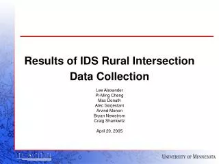
Results of IDS Rural Intersection Data Collection Lee Alexander Pi-Ming Cheng Max Donath Alec Gorjestani Arvind Menon Bryan Newstrom Craig Shankwitz April 20, 2005
Outline • Purpose • Data collection and archival • Data processing • Definition of gap • Results • General accepted gap analysis • Intersection zone analysis • Gaps as a function of time of day • Gaps for different vehicle maneuvers • Gaps as a function of vehicle classification • Waiting for a gap • Gaps as a function of weather conditions • Small accepted gap analysis • Conclusions
Purpose • Determine driver behavior at intersection • Measure actual accepted gaps in real traffic • Correlate accepted gap with other parameters to find relationships • Entry position • Maneuver type • Vehicle type • Waiting time • Weather • Use driver behavior results as design input to deployable IDS system (with DII)
Data Collection and Archival • 26 sensors at intersection • Radar, laser, image processing • Different data rates ( radar 10, laser 35, cameras 30 Hz) • Tracking software runs at deterministic 20 Hz • Estimates vehicle states using sensor data • “Snapshot” of intersection state at 10 Hz • Intersection state includes position, speed, lane, time to intersection of every vehicle in surveillance system coverage region
Data Collection and Archival • Hardware • Central control computer • Collects sensor data • Calculates vehicle states at 10 Hz • Sends vehicles states to data server • Image processor • Processes images from the four cameras at the intersection • Calculates vehicle positions • Data/web server computer • Hub for accessing real time data • Bridge between wired and wireless networks • Web server to share status information and images • Web Site • Intersection Data Acquisition System (iDAQ) • Video capture board • Captures four channels of MPEG layer 4 video • Engineering data • Removable hard drive bay
Data Collection and Archival • iDAQ • Receives images from four cameras • Digitizes and compresses to MPEG layer 4 video files • Recieves engineering data from Data Server (Ethernet) • Writes all video and data channels to removable SCSI disk drive
Data Processing • Hard drives couriered to the University every two weeks • Batch programs import data into database • Engineering data permanently stored, video files of interest stored, rest discarded • Data in raw format, needs to be processed to determine maneuvers • Creates intermediary databases • Contains Vehicles of Interest (VOI) • Vehicles accepting a gap • Zone and region location, times • Maneuvers assigned • Classification assigned (length, height) • Query program cross references database tables and produces reports
Definition of gap • Spatial database contains all relevant road features • Database divided into zones (entry regions) • Zones subdivided by regions(16 x 12 ft), within each lane • Sections assigned for each vehicle maneuver (right, left, straight) on each entry path • Time when vehicle leaves the designated region is when the gap is calculated • Gap associated with that point in time is used • Time for vehicle on major leg to arrive at the intersection if its speed and acceleration are held constant • Time gap used – normalizes speed • Primary gap – smallest gap to middle of intersection • Calculated for each lane • Captures gap when vehicle in harm’s way • Captures risk drivers accept
Definition of gap • Minor road vehicle (green) arrives at the intersection at time to • Minor road vehicle in section 114 at t1 • Major road vehicle (blue) is visible in section 10174 at t1 • Minor road vehicle completely leaves section 113 at t2 • Gap calculated at t2 • Gap time estimated by state of major road vehicle at t2
Results • Data collected from February 1 to March 29, 2005 • 24/7 • Over 9,000 measured gaps
All Accepted Gaps • Gaussian, mean 10.2s, median 9.7s • 10 seconds chosen as upper limit for lower gap statistics • 53% gaps less than 10 seconds • Mean gap 7.0 s for accepted gaps < 10 seconds • 5% of drivers accepted a gap of 4.4 s or less • 1% of drivers accepted a gap of 3.1 s or less
Intersection Zone Analysis • Zones encompass entry ways into major leg traffic • Used to determine maneuver type • Determine whether gap selection related to region where maneuver originates
Intersection Zone Analysis • Zones 1 and 8 have significantly smaller mean accepted gap time than zones 2 and 7 • Zones 1 and 8 have smaller variance than zones 2 and 7 • Vehicles in zones 1 and 8 merge/cross south bound traffic on US52 • Major leg (US52) traffic volumes similar in both directions
Intersection Zone Analysis • Sample surveillance system data every 10 sec for number of vehicles within surveillance system on Hwy 52 • South 2.9 vehicle detected per sample • North 3.1 vehicles detected per sample • STD 2.8 for north bound • STD 3.4 for south bound • Signalized intersection in Cannon Falls, 8 miles north • No signalized intersections in Zumbrota Falls, 12 miles south
Gaps as a Function of Time of Day • Gaps decrease during the day, largest at night • Smallest gaps accepted in evening rush • Largest gaps accepted at night time • Mean gap < 10 sec similar, slightly smaller for evening rush
Gaps as a Function of Time of Day • Lowest traffic volume at 10 UTC (6 AM CST) • Highest traffic rate at 23 UTC (5 PM CST) • Smallest gaps occur with largest traffic volume • No night time effect, day/night mean gap time < 10 s same
Gaps for different vehicle maneuvers • Few left hand turns • Largest accepted gap for left hand turns followed by right • Smallest accepted gap for straight through maneuvers
Gaps as a Function of Vehicle Classification • Four categories • Small passenger vehicles (motorcycles, sedans, small SUVs) • Large passenger vehicles (SUV, Pickups) • Small commercial vehicles (delivery trucks, dump trucks) • Large commercial vehicles (semi trucks) • No significant difference in accepted gap
Gaps as a Function of Vehicle Classification • Larger vehicles take longer to leave region due to their length and lower acceleration capabilities • Gap definition ignores time to accelerate and leave the stopped region • Larger vehicles decided (gap selection) to take the gap before smaller vehicles • Gap/Risk acceptance the same
Waiting For a Gap – Stop Bar • Total time spent in zone 1 or 2, stop bars • Peak at 12 seconds • Chose waiting periods based on histogram peak • 5 – 12 s • 12 – 17 s • 17 – 25 s • 25 – 60s
Waiting for a Gap – Stop Bar • Mean gap largest for vehicles waiting the least amount of time (5 – 12) • Median (50%) gaps similar • < 10s mean gap was lowest for 17-25 s wait, similar for other wait times
Waiting For a Gap – Cross Road (Median) • Half the vehicles spend less than 3.6s in cross roads • Time periods selected for analysis • 0 – 3 s • 3 – 5 s • 5 – 10 s • 10 – 60 s
Waiting for a gap – Cross Road (Median) • Mean accepted gap larger for shortest (0 – 3) and longest (10 – 60) wait times • < 10 s mean gap time similar, slightly smaller for longest wait • Vehicles that took the cross road as a one step maneuver (0 – 3 s) did not increase their risk
Gaps as a Function of Weather Conditions • ARWIS weather station located one mile north of intersection • Provides subsurface, surface and atmospheric data • Downloaded weather data nightly from a MNDOT web site • Visibility and precipitation rate was cross correlated with accepted gaps
Gaps as a Function of Weather Conditions - Visibility • Accepted gaps increased with decreasing visibility • < 10s mean gaps similar, similar risk • Speed on major leg decreased slightly as visibility decreased • Lower speed means larger gap time for same gap distance
Gaps as a Function of Weather Conditions – Precipitation Rate • Precipitation rate cross referenced with accepted gap • Mean gap increases with increasing precipitation rate • Speed decreases slightly with precipitation • High precipitation rate has lowest < 10s gap, but highest overall mean accepted gap
Small Accepted Gap Analysis • Need metric to demonstrate effectiveness of IDS system • Crashes are rare at any one intersection over small time sample • Use small (unsafe) gaps (< 4 sec) as measure of poor gap selection • If percentage of small gaps decrease, system shows positive effect on gap selection • 3.2% of accepted gaps were less than 4 sec • Maneuver type • 67% of all maneuvers were straight • 86% of all small gaps were straight • Zone • Zone 1: 16% of total, 20% of small gaps • Zone 2: 25% of total, 8% of small gaps • Zone 7: 33% of total, 20% of small gaps • Zone 8: 24% of total, 48% of small gaps • Classification type had similar representation of small gaps compared to total number of gaps • Vehicles performing straight maneuver across south bound lane of highway 52 from the median (zone 8) had highest percentage of small accepted gaps
Conclusions • Mean accepted gap for all vehicles was 10.2s • Mean accepted gap for gaps < 10 s was 7.0s • 5% gap was 4.4 s, 1% gap was 3.1 s • Vehicles crossing/merging south bound lanes of Hwy 52 had significantly smaller accepted gap than vehicles crossing/merging north bound lanes • Due to inconsistent traffic patterns, signalized intersections in Cannon Falls • Accepted gaps smaller with increasing traffic rate • Smallest at evening rush hour, largest at night time • Straight maneuvers exhibited smallest accepted gap, followed by right turn then left turn • Little difference in accepted gap between different vehicle classes
Conclusions • Gap definition did not take into account time to accelerate past the stop bar, larger vehicles likely selected a bigger gap • At stop bar, mean accepted gap largest for vehicles waiting the least time. <10s gap smallest for 17 – 25 s wait. • At cross roads, mean accepted gap smallest for vehicles waiting the shortest time (0 – 3) and vehicles waiting the longest (10 – 60). Little difference for gaps < 10s. • Mean gaps increased with decreasing visibility. Less significant for gaps < 10s. Speed on main leg decreased slightly with lower visibility. • Mean gaps increased with increasing precipitation rate. Little difference for gaps < 10s for precipitation rate < 0.9 cm/hr. Smaller gap for 0.9 to 1.5 cm/hr. • Small gap analysis (< 4s) showed that straight maneuvers over represented. • Vehicles crossing south bound 52 from median had greatest percentage of small gaps • 3.2% of accepted gaps were less than 4 sec