Download
1 / 25
250 likes | 354 Views
Blind Component Separation for Polarized Obseravations of the CMB. Jonathan Aumont, Juan-Francisco Macias-Perez. 24-03-2006. Rencontres de Moriond 2006 La Thuile, Italy. Overview. Model of the microwave sky Spectral matching algorithm extended to polarization Planck simulations

E N D
Blind Component Separation for Polarized Obseravations of the CMB Jonathan Aumont, Juan-Francisco Macias-Perez 24-03-2006 Rencontres de Moriond 2006 La Thuile, Italy
Overview Model of the microwave sky Spectral matching algorithm extended to polarization Planck simulations Performances of the algorithm Results Conclusions
Model of the microwave sky In real space: { I,Q,U }{ T,E,B } in Fourier space Data in the spherical harmonics space for X = { T,E,B }: Density matrices: Then data read:
Spectral matching • Expectation-Maximization (EM) algorithm [Dempster et al. JRSS 1977]: Set of parameters: q i = { RS ( l ), RN ( l ), A } • Iterations: • E-step: expectation of the likelihood for q i (gaussian prior) • M-step: maximization of the likelihood to compute q i+1 In this work, 10000 EM iterations are generally performed [Delabrouille, Cardoso & Patanchon, 2003, MNRAS]
Q Q Q I I I I, Q and U sky maps simulations • CMB • Spectra generated with CAMB [Lewis et al. ApJ 2000] for concordance model according to WMAP1 [Bennett et al. ApJS 2003], r = 0.7 and gravitational lensing • Thermal dust emission: • Power-law model • Normalized with respect to Archeops 353 GHz data [Ponthieu et al. A&A 2005] • Galactic synchrotron emission: • Template maps [Giardino et al. A&A 2002]: • Isotropic spectral index ( a = -2.7) White noise maps normalized to the instrumental noise level for each frequency
Priors and Planck Simulations • Blind analysis: • q ={ RS , RN , A } • no priors • Blind with A(T) = A(E) = A(B): • q= { RS , RN , A} • we suppose that emission laws are the same in temperature and polarization • Semi-Blind analysis: • q= { RS , RN , A(dust,sync)} • we suppose that the CMB electromagnetic spectrum is known and we fix it • Planck simulations: • LFI and HFI polarized channels: [30,40,70,100,143,217,353] GHz • 14 months nominal mission • complete sky coverage • infinite resolution • no systematics
Blind separation (CMB + Foregrounds + Noise) CMB + Synchrotron + Dust + Noise nside = 128 CMB BB EE TT EB TE TB Separation is efficient for TT, EE, TE, TB and EB No detection of BB modes Small bias in TT for l < 30
Blind separation (CMB + Foregrounds + Noise) (2) Dust TT BB EE EB TE TB Separation is efficient for TT, EE, BB, TE, TB, and EB
Blind separation (CMB + Foregrounds + Noise) (3) Synchrotron TT BB EE TB EB TE Separation is efficient for TT, EE, BB, TE, TB, and EB Small bias in TT for l < 50
Mixing matrix reconstruction (arbitrary units) Blind n (GHz) n (GHz) n (GHz) Blind, assuming T= E = B n (GHz) n (GHz) n (GHz) Dust Synchrotron CMB
Assuming A(T) =A(E) =A(B) (CMB + Foregrounds + Noise) CMB EE BB TT TB EB TE Detection of BB modes for l < 50 No bias at low l in TT
Semi-blind exploration of small angular scales (CMB + Fgds + Noise) nside = 512 CMB EE BB TT TE TB EB Reconstruction ofTT, TE, TB, EB up to l ~ 1500 Reconstruction of EE up to l ~ 1200 Reconstruction of BB up to l ~ 50
Error bars of the reconstruction CMB only / A fixed CMB + fgds / A(CMB) fixed CMB + fgds / Blind TT BB EE EB TB TE Presence of foregrounds increases the error bars by at least a factor of 2
Conclusions • Spectral matching algorithm extended to polarization to jointly deal with TT, EE, BB modes and also with cross power spectra TE, TB and EB We are able to separate blindly A, RN and RS, except for the CMB BB modes • When we suppose A(T) = A(E) = A(B) we are able to recover CMB BB modes for l < 50 at 5 s • Effect of the presence of foregrounds increases the error bars of the reconstruction. Decreases by addition of priors • Improvements: • beam smoothing • filtering smoothing • incomplete sky coverage effect • components with anisotropic spectral index [Aumont & Macias-Perez, 2006, submitted to MNRAS, astro-ph/0603044]
Model of the microwave sky (2) Example: 2 frequencies, 2 components data Density matrix expressions:
Bayes Theorem: Wiener solution: Formalism (2) Density matrices: Then data reads: Likelihood maximization
Sky maps simulations • CMB • Spectra generated with CAMB [Lewis et al. 2000] for concordance model with WMAP [Bennet et al. 2003] with gravitational lensing • Thermal dust emission: • Dust power-law model [Prunet et al. 1998] : • Normalized with respect to Archeops 353 GHz data [Ponthieu, …, Aumont et al. 2005] • Galactic synchrotron emission: • Template maps for I, Q and U [Giardino et al. 2002]: • Isotropic spectral index ( a =-2.7) White noise maps for each frequency
CMB power spectra • CMB: Spectra generated with CAMB [Lewis et al. 2000] for: • W0 = 1, WL= 0.7, Wm = 0.3, Wb = 0.046 • t = 0.17 • Gravitationnal lensing • r[10-4, 0.7]
The mixing matrix, A • Noise levels are relative noise levels with respect to the 143 GHz channel • At this frequency, noise levels are 6,3 mKCMB (T) and 12,3 mKCMB (E,B) per square pixels of side 7 arcmin and for a 14-months Planck survey
Blind reconstruction of the noise at 100 GHz Efficient reconstruction of the noise power spectra for T, E and B for nside= 512
Assuming A(T) =A(E) =A(B) (CMB + Foregrounds + Noise) Synchrotron EE BB TT TE TB EB No bias at low l in TT
Semi-blind exploration of small angular scales (CMB + Fgds + Noise) Dust nside = 512 EE BB TT TE TB EB Reconstruction ofTT, EE, BB, TE, TB, EB up to l ~ 1500
Semi-blind exploration of small angular scales (CMB + Fgds + Noise) Synchrotron nside = 512 EE BB TT TE TB EB Reconstruction ofTT, EE, BB, TE, TB, EB up to l ~ 1500
Reconstruction of the CMB BB modes (CMB + Fgds + Noise) A(CMB) fixed A fixed
Reconstruction of the CMB BB modes with SAMPAN Satellite prototype experiment with polarized bolometers at 100, 143, 217, 353 GHz Sensitivity 10 times better than Planck Simulations with CMB + Dust r = 10-2 r = 10-3 r = 10-1