Download
1 / 73
740 likes | 854 Views
Section 5.2 - Using Simulation to Estimate Probabilities.

E N D
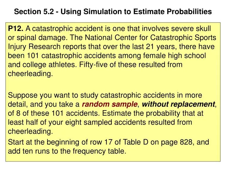
Section 5.2 - Using Simulation to Estimate Probabilities P12. A catastrophic accident is one that involves severe skull or spinal damage. The National Center for Catastrophic Sports Injury Research reports that over the last 21 years, there have been 101 catastrophic accidents among female high school and college athletes. Fifty-five of these resulted from cheerleading. Suppose you want to study catastrophic accidents in more detail, and you take a random sample, without replacement, of 8 of these 101 accidents. Estimate the probability that at least half of your eight sampled accidents resulted from cheerleading. Start at the beginning of row 17 of Table D on page 828, and add ten runs to the frequency table.
Section 5.2 - Using Simulation to Estimate Probabilities P12. Of the 101 catastrophic accidents among female high school and college athletes, 55 of resulted from cheerleading. Take a random sample, without replacement, of 8 of these 101 accidents. Estimate the probability that at least half of your eight sampled accidents resulted from cheerleading. Assumptions: You have a random sample (without replacement) of size n = 8 from a population of 101 accidents, of which 55 resulted from cheerleading. (Each sample of size n = 8 is equally likely.)
Section 5.2 - Using Simulation to Estimate Probabilities P12. Model: There are 1000 three-digit triples and you wish to represent 101 accidents, so it is convenient to assign 9 three-digit numbers to each accident, as follows. (If you assign the numbers 001 - 101, you will have to reject 90% of the numbers selected. This method rejects only 91 or 9.1%)
Section 5.2 - Using Simulation to Estimate Probabilities P12. Model: Assign 9 three-digit numbers to each accident, as follows. Ignore all triples not on the table. Accidents numbered from 1 through 55 will be considered as resulting from cheerleading. Stop a run when you have a sample of 8 accidents (no repeats). Repeat until you have 10 runs.
Section 5.2 - Using Simulation to Estimate Probabilities P12. Repetition: Starting on line 17 of Table D, divide the digits into triples. Triples to be ignored are crossed out and the remaining ones are grouped into sequences representing samples of 8 accidents, making sure there are no repeated accidents in any one run.
Section 5.2 - Using Simulation to Estimate Probabilities P12. Repetition:
Section 5.2 - Using Simulation to Estimate Probabilities P12. Repetition:
Section 5.2 - Using Simulation to Estimate Probabilities P12. Repetition:
Section 5.2 - Using Simulation to Estimate Probabilities P12. Repetition: Update Display 5.22
Section 5.2 - Using Simulation to Estimate Probabilities P12. Conclusion: Out of the 1000 runs, 722 samples had at least half (four or more) of the accidents from cheerleading. The estimated probability that a random sample of eight catastrophic accidents would have at least half of the accidents from cheerleading is about 0.722. This is close to the theoretical probability of 0.7374 computed using the hypergeometric distribution. See Fathom file SIA Ch 5 P12.ftm
Section 5.2 - Using Simulation to Estimate Probabilities P13. The winner of the World Series is the first team to win four games. That means the series can be over in four games or can go as many as seven games. Suppose the two teams playing are evenly matched. Estimate the probability that the World Series will go seven games before there is a winner. Start at the beginning of row 9 of Table D on page 828, and add your ten runs to the frequency table.
Section 5.2 - Using Simulation to Estimate Probabilities P13. The winner of the World Series is the first team to win four games. Suppose the two teams playing are evenly matched. Estimate the probability that the World Series will go seven games before there is a winner. Assumptions: The probability of a given team winning a particular game is 50% and that the results of the games are independent of each other. (This is probably not a realistic assumption!)
Section 5.2 - Using Simulation to Estimate Probabilities P13. Model: Assign digits 1-5 to team A winning and 6-9, 0 to team B winning. Select digits from the table, allowing repeats, until one of the teams has four wins. Record the total number of digits needed to get four wins for one of the teams.
Section 5.2 - Using Simulation to Estimate Probabilities P13. Repetition: Starting on line 09 of Table D:
Section 5.2 - Using Simulation to Estimate Probabilities P13. Repetition: Update Display 5.23
Section 5.2 - Using Simulation to Estimate Probabilities P13. Conclusion: Out of the 5000 runs, 1537 series went the full seven games, so the estimated probability of a World Series of two evenly matched teams going seven games is 1537 / 5000, or 0.3074. The theoretical probability is 0.3125. When the teams are not evenly matched, the probability is less. In the 66 World Series between 1940 and 2006, the World Series went the full seven games 27 times out of 66, or 0.409. This is not statistically significant, but close. One reasonable explanation is that the probability of winning changes from game to game.
Section 5.2 - Using Simulation to Estimate Probabilities E15. About 10% of high school girls report that they rarely or never wear a seat belt while riding in motor vehicles. Suppose you randomly sample four high school girls. Estimate the probability that no more than one of the girls says that she rarely or never wears a seat belt. Start at the beginning of row 36 of Table D on page 828, and add your ten results to the frequency table.
Section 5.2 - Using Simulation to Estimate Probabilities E15. About 10% of high school girls report that they rarely or never wear a seat belt while riding in motor vehicles. Suppose you randomly sample four high school girls. Estimate the probability that no more than one of the girls says that she rarely or never wears a seat belt. Assumptions: The probability that a randomly selected girl reports that she rarely or never wears a seat belt is 10%, and that the girls are selected independently of each other.
Section 5.2 - Using Simulation to Estimate Probabilities E15. Model: Assign the digits 0 to 9 as follows: Reports that she rarely or never wears a seat belt: 0 Does not report that she rarely or never wears a seat belt: 1-9
Section 5.2 - Using Simulation to Estimate Probabilities E15. Repetition: Begin with row 36 of table D, separated into groups of 4:
Section 5.2 - Using Simulation to Estimate Probabilities E15. Repetition: Add the results to the table in Display 5.24:
Section 5.2 - Using Simulation to Estimate Probabilities E15. Conclusion: Out of the 10,000 runs, 6641 + 2863 = 9504 had no more than one 0. The estimated probability that a random sample of four girls contains no more than one that says she rarely or never wears a seat belt is 0.9504 The theoretical probability is 0.9477.
Section 5.2 - Using Simulation to Estimate Probabilities E18. A Harris poll estimated that 25% of U.S. residents believe in astrology. Suppose you would like to interview a person who believes in astrology. Estimate the probability that you will have to ask four or more U.S. residents to find one who believes in astrology. Start at the beginning of row 15 of Table D on page 828, and add your ten results to the frequency table.
Section 5.2 - Using Simulation to Estimate Probabilities E18. A Harris poll estimated that 25% of U.S. residents believe in astrology. Suppose you would like to interview a person who believes in astrology. Estimate the probability that you will have to ask four or more U.S. residents to find one who believes in astrology. Assumptions: The probability that a randomly selected person believes in astrology is 25%, and that each person was selected randomly and independently from the population of U.S. residents.
Section 5.2 - Using Simulation to Estimate Probabilities E18. Model: Assign two digit-numbers as follows: Believes in astrology: 01 - 25 Does not believe in astrology: 26 - 99, 00
Section 5.2 - Using Simulation to Estimate Probabilities E18. Repetition: Begin with row 15 of table D:
Section 5.2 - Using Simulation to Estimate Probabilities E18. Repetition: Begin with row 15 of table D:
Section 5.2 - Using Simulation to Estimate Probabilities E18. Repetition: Add the results to the table in Display 5.24:
Section 5.2 - Using Simulation to Estimate Probabilities E18. Conclusion: Out of the 2,000 runs, 2000 - (437 + 413 + 282) = 868 had four or more. The estimated probability that you would have to interview four or more U.S. residents before getting a person who believes in astrology is 868 / 2000 or 0.434 The theoretical probability is 0.422. (You will learn how to compute this in Section 6.3)
Section 5.2 - Using Simulation to Estimate Probabilities E19. The probability that a baby is a girl is about 0.49. Suppose a large number of couples each plan to have babies until they have a girl. Estimate the average number of babies per couple. Start at the beginning of row 9 of Table D on page 828, and add your ten results to the frequency table in Display 5.28, which gives the results of 1990 runs.
Section 5.2 - Using Simulation to Estimate Probabilities E19. The probability that a baby is a girl is about 0.49. Suppose a large number of couples each plan to have babies until they have a girl. Estimate the average number of babies per couple. Assumptions: Each baby has a 0.49 chance of being a girl. The gender of each child is independent of the other children’s gender in that family.
Section 5.2 - Using Simulation to Estimate Probabilities E19. Model: Assign pairs of digits as follows: 01 - 49 = girl baby 50 - 99, 00 = boy baby A single run consists of selecting pairs of digits, allowing repeats, until a pair in the range 01 - 49 is selected. Record the number of pairs needed.
Section 5.2 - Using Simulation to Estimate Probabilities E19. Repetition: Start with Row 9 of Table D. Perform 10 repetitions. 63 / 57 / 33 // 21 // 35 // 05 // 32 // 54 / 70 / 48 // 90 / 55 / 35 // 75 / 48 // 28 // 46 // The numbers needed are: 3, 1, 1, 1, 1, 3, 3, 2, 1, 1
Section 5.2 - Using Simulation to Estimate Probabilities E19. Repetition: Add the results of our ten runs to the frequency table:
Section 5.2 - Using Simulation to Estimate Probabilities E19. Conclusion: Apply the method of calculating a mean from a frequency table: Enter the data into L1, L2; Run 1-Var Stats.
Section 5.2 - Using Simulation to Estimate Probabilities E19. Conclusion: Apply the method of calculating a mean from a frequency table: Enter the data into L1, L2; Run 1-Var Stats. The estimated average number of babies for a family that keeps having babies until they have a girl is about 2.122 children. The theoretical mean is about 2.04.
Section 5.2 - Using Simulation to Estimate Probabilities E20. Boxes of cereal often have small prizes in them. Suppose each box of one type of cereal contains one of four different small cars. Estimate the average number of boxes a parent will have to buy until his or her child gets all four cars. Start at the beginning of row 49 of Table D on page 828, and add your ten results to the frequency table.
Section 5.2 - Using Simulation to Estimate Probabilities E20. Boxes of cereal often have small prizes in them. Suppose each box of one type of cereal contains one of four different small cars. Estimate the average number of boxes a parent will have to buy until his or her child gets all four cars. Assumptions: The different types of cars are equally and randomly distributed in the boxes of cereal so the probability if getting a particular type of car is always 0.25. Each box of cereal is selected independently.
Section 5.2 - Using Simulation to Estimate Probabilities E20. Model: Assign two digit-numbers as follows: Car 1: 01 - 25 Car 2: 26 - 50 Car 3: 51 - 75 Car 4: 76 - 99, 00
Section 5.2 - Using Simulation to Estimate Probabilities E20. Repetition: Begin with row 49 of table D:
Section 5.2 - Using Simulation to Estimate Probabilities E20. Conclusion:
Section 5.2 - Using Simulation to Estimate Probabilities E20. Conclusion: We were asked to estimate a mean, not a probability. Count 27+ as 27.
Section 5.2 - Using Simulation to Estimate Probabilities E20. Conclusion: We were asked to estimate a mean, not a probability. The estimated mean number of boxes a parent must buy to get all four cars is 8.3402.
Section 5.2 - Using Simulation to Estimate Probabilities E21. A group of five friends have backpacks that all look alike. They toss their backpacks on the ground and later pick up a backpack at random. Estimate the probability that everyone gets his of her own backpack. Start at the beginning of row 31 of Table D on page 828.
Section 5.2 - Using Simulation to Estimate Probabilities E21. A group of five friends have backpacks that all look alike. They toss their backpacks on the ground and later pick up a backpack at random. Estimate the probability that everyone gets his of her own backpack. Assumptions: Each backpack is equally likely to be picked up by each person. The backpacks are selected independently of each other.
Section 5.2 - Using Simulation to Estimate Probabilities E21. Model: Backpack 1 belongs to person 1, backpack 2 belongs to person 2, etc. Assign digits to represent backpacks: digits 1 and 2 = backpack 1; digits 3 and 4 = backpack 2; digits 5 and 6 = backpack 3; digits 7 and 8 = backpack 4; digits 9 and 0 = backpack 5. Select 4 digits and ignore repeats. Record the number of correct backpacks.
Section 5.2 - Using Simulation to Estimate Probabilities E21. Repetition: Begin with row 31 of table D. Perform 20 repetitions. 0449352 / 49475 / 246338 / 24458 / 6251025619627 / 933565337 / 124720 / 054997 / 65464051 / 88159 / 9611963 / 89654 / 6928 / 23912328 / 7295 / 2935 / 9631 / 5307 / 2689 / 80935
Section 5.2 - Using Simulation to Estimate Probabilities E21. Repetition:
Section 5.2 - Using Simulation to Estimate Probabilities E21. Repetition:
Section 5.2 - Using Simulation to Estimate Probabilities E21. Repetition: