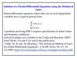
Method of Lines
460 likes | 605 Views
Method of Lines. Outline. This topic introduces the method of lines Used for solving heat-conduction/diffusion and wave equations Finite differences discretizes both time and space Discretize only space Use a high-quality ODE solver to find the solution over time.

Method of Lines
E N D
Presentation Transcript
Outline This topic introduces the method of lines • Used for solving heat-conduction/diffusion and wave equations • Finite differences discretizes both time and space • Discretize only space • Use a high-quality ODE solver to find the solution over time
Outcomes Based Learning Objectives By the end of this laboratory, you will: • You will understand the method of lines • You will be able to implement it using the Matlab functions implemented in previous terms
Integration-by-Parts in Higher Dimensions Up to this point, we have discretized both the space and time dimensions • We will look at another approach that discretizes only the space dimensions
Discretizing in Space Consider the heat-conduction/diffusion equation Discretizing the space component in one dimension gives: We will demonstrate this only in one dimension; however, the generalization to 2 and 3 dimensions is obvious…
Discretizing in Time With finite differences, we divided time into discrete steps, as well: which allowed us to find
Review of Finite Differences We are given the initial state of the system by uinit(x) Divide the space interval into n points with n – 1 intervals
Review of Finite Differences We evaluate the initial state at each of the n points
Review of Finite Differences Next, given these initial values, we take the finite-difference equation to approximate the state at the next time t2 = t1 + Dt equatio • The boundary values are defined by functions a(t) and b(t)
Review of Finite Differences Now, with this approximation, we approximate the values at timest3, t4, etc.
Method of Lines As an alternative approach, associate with each spatial point an unknown function uk(t) • Two exceptions: u1(t) = a(t) un(t) = b(t) This approach was popularized by the chemical engineer William E. Schiesser in his 1991 text The Numerical Method of Lines
Method of Lines In order to substitute uk(t) into our mixed partial-/finite-difference equation, we note that the solution at location x – his uk – 1(t) and the solution at x + his uk + 1(t): We also have the initial condition: uk(tinitial) = uinit(xk)
Systems of IVPs Therefore, we have a system of n – 2 initial-value problems but with n unknown functions:
Systems of IVPs There are two unknown functions, however, these are given by our boundary conditions:
Systems of IVPs We therefore have a systemof n – 2 initial-value problems • With n = 9:
Systems of IVPs Note that we can rewrite the differential equations: Thus,
Systems of IVPs We can therefore write this as: where
IVP Solvers from Previous Courses From MATH 211, you implemented the function function [ ts, ys ] = dp45n( f, t_int, y1, h, eps_step) where tint = [tinitial, tfinal] that uses the adaptive Dormand-Prince method to approximate a solution to a system of initial-value problems where we allow a maximum error of estep where we start with an initial step size in time of h starting at tinitial and going to tfinal
IVP Solvers from Previous Courses We can write the function function du = f( t, u ) M = diag( -2*ones( n - 2, 1 ) ) + ... diag( ones( n - 3, 1 ), 1 ) + ... diag( ones( n - 3, 1 ), -1 ); du = (kappa/h^2)*(M*u + [a(t); zeros( n – 4, 1 ); b(t)]); end
Example: Dirichlet Conditions To give a specific example, consider the following heat-conduction/diffusion problem: that is, k = 0.2, on [0, 1] with with n = 9 points
Example: Dirichlet Conditions To give this a description: • A bar is initial uniform at 1 • For the first second, the left-hand side is placedin contact with a heat sink at 0, after which itis switched with a heat source of 2 • For the first two seconds, the right-hand sideis in contact with a body also at 1, after whichit is switched with a heat sink at 0
Example: Dirichlet Conditions Thus, we have: function du = f111( t, u ) n = 9; M = diag( -2*ones( n - 2, 1 ) ) + ... diag( ones( n - 3, 1 ), 1 ) + ... diag( ones( n - 3, 1 ), -1 ); kappa = 0.2; h = 1/8; a = @(t)(2*(t > 1)); b = @(t)(t < 2); du = (kappa/h^2)*(M*u + [a(t); zeros( n - 4, 1 ); b(t)]); end
Example: Dirichlet Conditions This can be driven by: u_init = @(x)(x*0 + 1); a = @(t)(2*(t > 1)); b = @(t)(t < 2); n = 9; xs = linspace( 0, 1, n )'; [ts, us] = dp45( @f111, [0, 3], u_init( xs(2:end - 1) ), 1, 0.0001); us = [a(ts); us; b(ts)]; mesh( ts, xs, us );
Example: Dirichlet Conditions With two orientations, the output is the plot:
Example: Dirichlet Conditions Note that Dt is larger while the system converges but becomes smaller at the discontinuities
Example: Insulated Conditions To give a specific example, consider the following heat-conduction/diffusion problem: that is, k = 0.2, on [0, 1] with and an insulated right-hand boundary with n = 9 points
Example: Insulated Conditions Using the 2nd-order divided difference approximation of the derivative: and substituting our approximations for u(b, t), u(b – h, t), andu(b – 2h, t) equate this to zero, we have: or
Example: Insulated Conditions We could then substitute into the last equation to get
Example: Insulated Conditions Thus, we have: function du = f112( t, u ) n = 9; M = diag( -2*ones( n - 2, 1 ) ) + ... diag( ones( n - 3, 1 ), 1 ) + ... diag( ones( n - 3, 1 ), -1 ); M(n - 2, n - 2) = -2/3; M(n - 2, n - 3) = 2/3; kappa = 0.2; h = 1/8; a = @(t)(t > 1); du = (kappa/h^2)*(M*u + [a(t); zeros( n - 4, 1 ); 0]); end Recall:
Example: Insulated Conditions This can be driven by: u_init = @(x)(x*0 + 1); a = @(t)(t > 1); n = 9; xs = linspace( 0, 1, n )'; [ts, us] = dp45( @f111, [0, 3], u_init( xs(2:end - 1) ), 1, 0.0001); us = [a(ts); us; (4*us(end,:) - us(end - 1,:))/3]; mesh( ts, xs, us );
Example: Insulated Conditions With two orientations, the output is the plot:
Example: Neumann Conditions Suppose that the right-hand side is a more general Neumann condition: Again, use the approximation and substituting our approximations for u(b, t), u(b – h, t), andu(b – 2h, t) equate this to zero, we have: or
The Wave Equation We can also have an initial-value problem for the wave equation: This can, of course, be generalized to two and three dimensions: • There is one unknown function for each point
The Wave Equation Recall that our function dp45.m only works with a 1st-order differential equation • We must therefore convert the 2nd-order ODE into a 1st-order ODE
The Wave Equation We therefore have a systemof 2(n – 2) initial-value problems • With n = 9:
The Wave Equation Note that we can rewrite the differential equations:
The Wave Equation We can therefore write this with :
The Wave Equation Where the function f is defined as:
The Wave Equation Thus, we have: function [dw] = f113( t, w ) n = 17; c = 1; h = 1/8; r = (c/h)^2; Id = ones( n - 2, 1 ); Id_off = ones( n - 3, 1 ); Z = zeros( n - 2, n - 2 ); M = diag( -2*r*Id ) + diag( r*Id_off, 1 ) + diag( r*Id_off, -1 ); M = [Z eye( n - 2, n - 2 ); M Z]; v = zeros( 2*n - 4, 1 ); a = @(t)(sin(3*t)); b = @(t)(0*t); v(n - 1) = r*a(t); v(end) = r*b(t); dw = M*w + v; end
The Wave Equation This can be driven by: u_init = @(x)(x*0); du_init = @(x)(x*0); a = @(t)(sin(3*t)); b = @(t)(0*t); n = 17; xs = linspace( 0, 1, n )'; U_init = [u_init( xs(2:end - 1) ); du_init( xs(2:end - 1) )]; [ts, us] = dp45( @f113, 0, 10, U_init, 1, 0.0001); size( us ) u = [a(ts); us(1:(n - 2), :); b(ts)]; mesh( ts, xs, u ); du = [cos(3*ts); us((n - 1):end, :); 0*ts]; % Plot the derivative... mesh( ts, xs, du );
The Wave Equation The plot of the solution and the derivative are here:
Finite Element Methods It will also work equally effectively for finite element methods: • The elements define the relationship between a function defined at a point and its neighbouring functions
Summary In this topic, we have covered the method of lines: • We discretize only the space component • This creates a system of initial-value problems • This may be solved using a high-accuracy adaptive ODE solver
References [1] Schiesser, W. E., The Numerical Method of Lines, Academic Press, 1991.
Usage Notes • These slides are made publicly available on the web for anyone to use • If you choose to use them, or a part thereof, for a course at another institution, I ask only three things: • that you inform me that you are using the slides, • that you acknowledge my work, and • that you alert me of any mistakes which I made or changes which you make, and allow me the option of incorporating such changes (with an acknowledgment) in my set of slides Sincerely, Douglas Wilhelm Harder, MMath dwharder@alumni.uwaterloo.ca