Download
1 / 12
120 likes | 146 Views
Learn about Principal Component Analysis (PCA) and its applications. Discover how PCA works, finding principal components, batch and online learning methods, kernel PCA, and Canonical Correlation Analysis. Explore PCA's role in feature extraction, data preprocessing, and image interpretation.

E N D
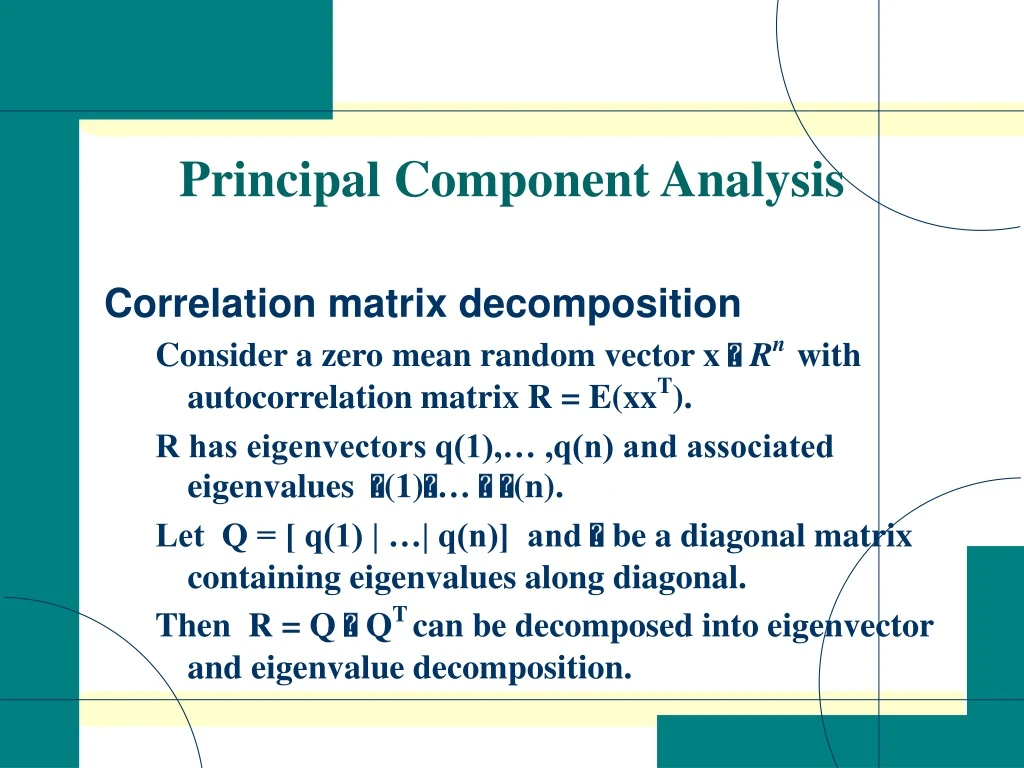
Principal Component Analysis Correlation matrix decomposition Consider a zero mean random vector x Rn with autocorrelation matrix R = E(xxT). R has eigenvectors q(1),… ,q(n) and associated eigenvalues (1)… (n). Let Q = [ q(1) | …| q(n)] and be a diagonal matrix containing eigenvalues along diagonal. Then R = Q QT can be decomposed into eigenvector and eigenvalue decomposition.
PCA works with data x x x x x x x x x x x x x x x x x x x x Given (x(1),x(2),…,x(m)) find weight direction that gives most information about data.
First Principal Component Let X= [ x(1) | …| x(m)] and R= (1/m)XXT (sample correlation matrix). Problem: max wTRw subject to ||w||=1. Maximum obtained when w= q(1) as this corresponds to wTRw = (1). q(1) is first principal component of x and also yields direction of maximum variance. y(1) = q(1)T x is projection of x onto first principal component. x q(1) y(1)
Other Principal Components ith principal component denoted by q(i) and projection denoted by y(i) = q(i)T x with E(y(i)) = 0 and E(y(i)2)= (i). y(i) Note that y= QTx and we can obtain data vector x from y by noting that x=Qy. We can approximate x by taking first m principal components (PC) to get z: z= q(1)x(1) +…+ q(m)x(m). Error given by e= x-z. e is orthogonal to q(i) when 1 i m. All PCA give eigenvalue / eigenvector decomposition of R and is also known as the Discrete Karhunen Loeve Transform
Diagram of PCA x x x x x Second PC x x x First PC x x x x x x x x x x x x First PC gives more information than second PC.
Learning Principal Components • Given m inputs (x(1), x(2), … x(m)) how can we find the Principal Components? • Batch learning: Find sample correlation matrix 1/m XTX and then find eigenvalue and eigenvector decomposition. Decomposition can be found using SVD methods. • On-line learning: Oja’s rule learns first PCA. Generalized Hebbian Algorithm, APEX.
PCA and LS-SVM formulation Problem: max wTXXTw subject to wTw=1. Reformulated in terms of SV QP methods: max J(w,e) = /2 eTe - 1/2 wTw Subject to e= XTw Lagrangian becomes max L(w,e,) = /2 eTe - 1/2 wTw - T(e- XTw) Take derivatives wrt each variable and set to zero to get that w= X, = e, and e- XTw = 0. Eliminate e and w to get that / - XTX = 0
Dual Space Formulation and Comments • Let K = XTX and = 1/, then we have an eigenvalue/ eigenvector problem in dual space, K = . • Want to maximize eTe = T/2 = max when eigenvectors are normalized to have magnitude 1. • Problem can easily be modified if data does not have zero mean and also to include bias term. • Convergence to first eigenvector of ensemble correlation matrix • Fisher Discriminant Analysis (FDA) (similar to PCA except FDA has targets to minimize scatter around targets)
Kernel Methods In many classification and detection problems a linear classifier is not sufficient. However, working in higher dimensions can lead to “curse of dimensionality”. Solution: Use kernel methods where computations done in dual observation space. X X O X O O X O Input space Feature space : X Z
Kernel PCA • Obtain nonlinear features from data • Can form kernel PCA in primal space (R) or dual space (K). • Problem closely related to LS SVM • Must ensure feature data has zero mean • Applications: Preprocessing data, denoising, compression, image interpretation
KPCA Formulation • Kernel PCA uses kernels to max E(0-wT ((x) - m ))2. • Use input data to approximate ensemble average to get the following quantities,(x) = ((x(1), …, (x(m))T , R is sample covariance matrix, and kernel matrix is K= ((x) – 1/m 11T (x))((x) – 1/m 11T (x))T • We can formulate as a QP problem where we max ½wT Rw subject to wT w = 1 and w= ((x) – 1/m 11T (x)) T • Can solve in primal or dual spaces. In dual space we have another eigenvector /eigenvalue problem K = .
Canonical Correlation Analysis • Given two pairs of data, can we extract features from different data. • Problem: Given x Rn1 and y Rn2 are zero mean vectors , find zx= wTx and zy=vTy so that correlation defined by (zx,zy) = E(zxzy)/(E(zx,zx)E(zyzy))½ is maximized. • QP formulation: max J(w,v) = wTCxy v subject to wTCxx w = 1 and vTCyy v = 1 where Cxx = E(xxT), Cyy = E(yyT), and Cxy = E(xyT). • CCA can be formulated using dual space and kernel CCA can also be constructed.


