Download
1 / 38
380 likes | 515 Views
Does the distribution have one or more peaks (modes) or is it unimodal? Is the distribution approximately symmetric or is it skewed in one direction? Is it skewed to the right (right tail longer) or left?. Example Description.

E N D
Does the distribution have one or more peaks (modes) or is it unimodal? • Is the distribution approximately symmetric or is it skewed in one direction? Is it skewed to the right (right tail longer) or left?
Example Description • Shape: The distribution is roughly symmetric with a single peak in the center. • Center: You can see from the histogram that the midpoint is not far from 110. The actual data shows that the midpoint is 114. • Spread: The spread is from 80 to about 150. There are no outliers or other strong deviations from the symmetric, unimodal pattern.
Calculator Example Text (To save data for later use on home screen type L1 -> Prez)
Calc continued • Frequency shortcut: If you have a dataset comprised of 75 3’s and 35 4’s for example, you can enter the values in list 1 and the frequencies in list 2 then pull 1 variable stats: • Stats-edit- L1: 3, 4 L1: 75, 35 stat-calc-1var stats L1,L2 enter
Relative frequency/Cumulative Frequency • A histogram does a good job of displaying the distribution of values of a quantitative variable, but tells us little about the relative standing of an individual observation. • So, we construct an ogive (“Oh-Jive”) aka a relative cumulative frequency graph.
Step 1- Construct table • Decide on intervals and make a frequency table with 4 columns: Freq, Relative frequency, cumulative frequency, and rel. cum. Freq. • To get the values in the rel. freq. column, divide the count in each class interval by the total number of observations. Multiply by 100 to convert to %. • In Cum freq column, add the counts that fall in or below the current class interval • for rel. cum. freq. column, divide the entries in the cum freq column by total number of individuals.
Step 2 & 3 • Label and scale your axes and title your graph. Vertical axis always Relative Cum. Freq. Scale the horizontal axis according to your choice of class intervals and the vertical axis from 0% to 100%. • Plot a point corresponding to the rel. Cum. freq. in each class interval at the LEFT ENDPOINT of the NEXT class interval. (example, the 40 to 44 interval, plot a point at a height of 4.7% above the age value of 45. • Begin with 0% you should end with 100%. Connect dots
To Locate an individual within distribution: What about Clinton? He was 46. To find his relative standing, draw a vertical line up from his age (46) on the horizontal axis until it meets the ogive. Then draw a horizontal line from this point of intersection to the vertical axis. Based on our graph his age places him at the 10% mark which tells us that about 10% of all US presidents were the same age as or younger than Bill Clinton when they were inaugurated. To locate a value corresponding to a percentile, do the opposite. Ex: 50th percentile, 55 years old.
Whenever data are collected over time, plot observations in time order. Displays of distributions such as stemplots and histograms which ignore time order can be misleading when there is systematic change over time.
Exploring Data • 1.2 Describing Distributions with Numbers • YMS3e • AP Stats at CSHNYC • Ms. Namad
Shape? Outliers? Center? Spread? Sample Data • Consider the following test scores for a small class: Plot the data and describe the SOCS: What number best describes the “center”? What number best describes the “spread’?
Measures of Center • Numerical descriptions of distributions begin with a measure of its “center”. • If you could summarize the data with one number, what would it be? Mean: The “average” value of a dataset. Median: Q2 or M The “middle” value of a dataset. Arrange observations in order min to max Locate the middle observation, average if needed.
Mean vs. Median • The mean and the median are the most common measures of center. • If a distribution is perfectly symmetric, the mean and the median are the same. • The mean is not resistant to outliers. • You must decide which number is the most appropriate description of the center...
Measures of Spread • Variability is the key to Statistics. Without variability, there would be no need for the subject. • When describing data, never rely on center alone. • Measures of Spread: • Range - {rarely used...why?} • Quartiles - InterQuartile Range {IQR=Q3-Q1} • Variance and Standard Deviation {var and sx} • Like Measures of Center, you must choose the most appropriate measure of spread.
med Q3=29.5 Q1=23 Q1 Q3 med=79 Quartiles • Quartiles Q1 and Q3 represent the 25th and 75th percentiles. • To find them, order data from min to max. • Determine the median - average if necessary. • The first quartile is the middle of the ‘bottom half’. • The third quartile is the middle of the ‘top half’.
45 50 55 60 65 70 75 80 85 90 95 100 Quiz Scores Outlier? 5-Number Summary, Boxplots • The 5 Number Summary provides a reasonably complete description of the center and spread of distribution • We can visualize the 5 Number Summary with a boxplot.
Determining Outliers “1.5 • IQR Rule” • InterQuartile Range “IQR”:Distance between Q1 and Q3. Resistant measure of spread...only measures middle 50% of data. • IQR = Q3 - Q1 {width of the “box” in a boxplot} • 1.5 IQR Rule:If an observation falls more than 1.5 IQRs above Q3 or below Q1, it is an outlier. Why 1.5? According to John Tukey, 1 IQR seemed like too little and 2 IQRs seemed like too much...
1.5 • IQR Rule • To determine outliers: • Find 5 Number Summary • Determine IQR • Multiply 1.5xIQR • Set up “fences” Q1-(1.5IQR) and Q3+(1.5IQR) • Observations “outside” the fences are outliers.
fence: 19.06-39.99 = -20.93 outliers IQR=45.72-19.06 IQR=26.66 fence: 45.72+39.99 = 85.71 0 10 20 30 40 50 60 70 80 90 100 Spending ($) { } Outlier Example All data on p. 48. 1.5IQR=1.5(26.66) 1.5IQR=39.99
Standard Deviation • Another common measure of spread is the Standard Deviation: a measure of the “average” deviation of all observations from the mean. • To calculate Standard Deviation: • Calculate the mean. • Determine each observation’s deviation (x - xbar). • “Average” the squared-deviations by dividing the total squared deviation by (n-1). • This quantity is the Variance. • Square root the result to determine the Standard Deviation.
Standard Deviation • Variance: • Standard Deviation: • Example 1.16 (p.85): Metabolic Rates
Standard Deviation Metabolic Rates: mean=1600 What does this value, s, mean?
Linear Transformations • Variables can be measured in different units (feet vs meters, pounds vs kilograms, etc) • When converting units, the measures of center and spread will change. • Linear Transformations (xnew=a+bx) do not change the shape of a distribution. • Multiplying each observation by b multiplies both the measure of center and spread by b. • Adding a to each observation adds a to the measure of center, but does not affect spread.
Data Analysis Toolbox To answer a statistical question of interest: • Data: Organize and Examine • Who are the individuals described? • What are the variables? • Why were the data gathered? • When,Where,How,By Whom were data gathered? • Graph: Construct an appropriate graphical display • Describe SOCS • NumericalSummary: Calculate appropriate center and spread (mean and s or 5 number summary) • Interpretation: Answer question in context!
Chapter 1 Summary • Data Analysis is the art of describing data in context using graphs and numerical summaries. The purpose is to describe the most important features of a dataset.