What we have now:
660 likes | 757 Views
What we have now:. Data:. Theory: Born Approximation model , Parratt’s theory , Sinha’s DWBA (including calculation for Yoneda wings). The rule we and our codes followed:. Experimental measured intensity:. Depends on surface tension γ !. Resolution function is very important!.

What we have now:
E N D
Presentation Transcript
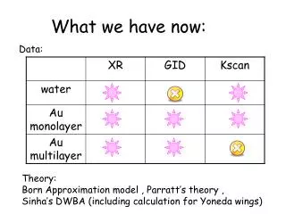
What we have now: Data: Theory: Born Approximation model , Parratt’s theory , Sinha’s DWBA (including calculation for Yoneda wings)
The rule we and our codes followed: Experimental measured intensity: Depends on surface tensionγ! Resolution function is very important! Constant for K-scan! (constant qz)
Au monolayer reflectivity fitting With our fitting code,we’re able to fit the reflectivity very well even for Au multilayer,but always get negative density part due to the broadening of error functions.
Fitting resolution function(fixed γ=72 mN/m):Blue – fixed Vert. Slit(0.52mm),Hori. Slit(1.89mm) (sli=[11,3])Red – fitted Vert. Slit(0.53mm),Hori. Slit(3.59mm) Resolution function calculated from slits size needs to be corrected? Water kscan '63-69‘ Qz=0.22 Even water can not be reproduced well. (due to temperature change or pollution?)
Water '71-77', sli=[11,3],bac=0.5 ,Qz=0.33 Unknown peak presents at Q~0.073, The position doesn’t change with γ. Fitting resolution function:Blue – fixed Vert. Slit(0.52mm),Hori. Slit(1.89mm)Red – fitted Vert. Slit(0.52mm),Hori. Slit(3.61mm)
Water '79-106', sli=[11,3],bac=0.5 ,Qz=0.44 Need to figure out! The slit size Vert.=0.52 Hori.=1.89 could fit the data perfectly.No cerrection to resolution function.And slit(0.52,3.60) seems also work not bad.
Do we need to correct our resolution function from slit (0.52,1.89) to slit (0.52,3.6)? Reason?
Big problem: Ununiformity of sample (beam damage?)& Lack of reproducibility Three data sets for Qz=0.22 are different from each other –monolayer is not reproducible…black—148(w/thoils ), red—217 blue– 273
Surface tension rules! monoAu ‘217-', sli=[11,3],bac=0.5 ,Qz=0.22 Highly depends on surface tension blue-- γ =18 (~heptane) magenta–-γ=30 red–- γ=72(water)
Surface tension fitting(with fixed slit0.52,1,89) monoAu ‘217-', sli=[11,3],bac=0.5 ,Qz=0.22 fitted γ=45 mN/m (between water 72 & Heptane ~20)
monoAu ‘313-', sli=[11,3],bac=0.5 ,Qz=0.33 fitted γ=45 mN/m
monoAu ‘299-', sli=[11,3],bac=0.5 ,Qz=0.44 fitted γ=48 mN/m
Can we make samples more uniform and reproducible? Contains information about the property and structure of the Au nanoparticle films? Are we able to fit this part by modifying our codes? Due to the surface tension difference between water and solvent for nanoparticle? Should we compare it to thin solvent material film on water surface?
After compression(compared to uncompressed results) Au 331,Qz=0.22 , red-- fitted γ=31 mN/m blue-- uncompressed γ=45 mN/m Au 345 Qz=0.44 , red--fitted γ=38 mN/m blue—uncompressed γ=48 mN/m
How does the compression lower surface tention of this system? Through increasing thickness of the solvent or increasing density of nanoparticles?
Water sample 3 :k scan 133-139,Qz=0.22s1=[1,0.04]mm,slit=[11,3]pixels, γ=72,65,60mN/m
Water sample 2: k scan 71-77,Qz=0.33s1=[1,0.06]mm, slit=[11,3]pixels, γ=72,65,60mN/m
Water sample2 :k scan 79-106,Qz=0.44s1=[1,0.06]mm, slit=[11,3]pixels, γ=72mN/m
Water sample 3 : k scan 133-139,Qz=0.22s1=[1,0.04]mm,slit=[22,3]pixels, γ=72,65,60mN/m
Water sample 2 : k scan 71-77,Qz=0.33s1=[1,0.06]mm,slit=[22,3]pixels, γ=72,65,60mN/m
Water sample 2 : k scan 79-106,Qz=0.44s1=[1,0.06]mm,slit=[22,3]pixels, γ=72,65,60mN/m
Au sample 2 : k scan 217-241,Qz=0.22s1=[1,0.04]mm,slit=[11,3]pixels, γ=45mN/m
Change in horizontal electronic slitWater sample 3 :k scan 133-139,Qz=0.22
Change in vertical electronic slitWater sample 3 :k scan 133-139,Qz=0.22
Water sample 3 : k scan 133-139,Qz=0.22s1=[1,0.04]mm,slit=[22,3]pixels, γ=72mN/m
Water sample 2 : k scan 71-77,Qz=0.33s1=[1,0.06]mm,slit=[22,3]pixels, γ=72N/m
Water sample 2 : k scan 79-106,Qz=0.44s1=[1,0.1]mm,slit=[22,3]pixels, γ=72mN/m
Au sample 2 : k scan 217-241,Qz=0.22s1=[1,0.04]mm,slit=[11,3]pixels, γ=45mN/m
Oct2008 sample 2,Au monolayer Kscan Qz=0.22(#217),0.33(#313),0.44(#299)sli=[11,3]pix,s1=[1,0.04/0.12]mm, γ=45mN/m
Aug2008 sample 1, Au monolayer reflectivity fitting right figure shows the corresponding electron density profile (smoothing parameter σ=6)
Aug2008 sample 1, Au monolayer beta-scan(#91-95)changing smoothing parameter σ=6(top)3(bottom)right panel shows the corresponding electron density profile
Aug2008 sample 1, Au monolayer beta-scan(#91-95)α=1.866,smoothing parameter σ=3right panel shows the difference between data and fitting (data/fitting)
Aug2008 sample 1, Au monolayer beta-scan(#97-101)α =2.488,smoothing parameter σ=3right panel shows the difference between data and fitting (data/fitting)
Aug2008 sample 1, Au monolayer beta-scan(#102-111)α =3.111,smoothing parameter σ=3right panel shows the difference between data and fitting (data/fitting)
Aug2008 sample 1, Au monolayer beta-scan(#91-95)changing smoothing parameter σ=3 2.8The decay curves show the beta-scan fitting without structure factor
Aug2008 sample 3, Au multilayer beta-scan(#251-254)α=1.696,γ=72(cyan),60(red) mN/m peak in a bump can’t fit…
Aug2008 sample 3, Au multilayer beta-scan(#255-260)α=2.262,γ=45(blue),60(red) mN/m When the specular peak is merged in a bump of structure factor, it’s difficult to fit the vicinity of the peak.


