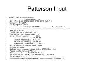
Patterson Input
Patterson Input. The CRYSDA file has been created : a print is given in LIS2 Cell 7.756 10.535 10.786 109.92 97.75 102.77 SpGr P -1 Formula C14 H18 O8 Mn1 End of program DDSTART

Patterson Input
E N D
Presentation Transcript
Patterson Input • The CRYSDA file has been created • : a print is given in LIS2 • Cell 7.756 10.535 10.786 109.92 97.75 102.77 SpGr P -1 • Formula C14 H18 O8 Mn1 • End of program DDSTART • ============ Execute program DDMAIN ============ for compound: XL • ================================================================ XL • RUN TITLE: xl in P-1 • First MERBIN use as subroutine: 1997 • Input data file: FREF Header: FREF xl • Number of input reflections: 3689 • Maximum indices output: 10 13 13 • Minimum indices output: 0 -13 -14 • HKLmax incl. symmetry: 10 13 14 • Maximum sin(TH/LAMBDA): 0.65853 • Number of reflections (merged) output: 3689 • WILSON plot results • Scale and overall temperature factor: Scale = 0.73339 Bov: 1.969 • Prepare input for sharpened Patterson • Origin removed sharpened PATTERSON function • (( 0.7334*Fobs)**2 - ORIGIN) * (0.2+STL)**2 * exp( 1.969*STL2) • End of program DDMAIN • ============ Execute program FOUR ============ for compound: XL
Patterson Output • ================================================================ XL • RUN TITLE: xl in P-1 • Sharpened Patterson for program PATTY • Patterson peak coordinates written to file ATOMS • List of ten highest Patterson peaks and their vector length • Peak height x y z length • 1 6000. 0.0000 0.0000 0.0000 0.00 • 2 1810. 0.4465 0.1687 0.0391 3.42 • 3 884. 0.1943 0.0299 -0.1257 2.20 • 4 819. 0.2839 -0.2987 -0.1239 4.19 • 5 808. -0.1251 0.1590 -0.0419 2.25 • 6 789. 0.2818 0.1316 0.0887 2.19 • 7 789. -0.4815 0.1180 -0.1629 4.51 • 8 757. -0.4387 0.0092 0.0798 3.63 • 9 742. -0.3220 0.1626 -0.1813 3.98 • 10 712. 0.1257 0.3283 -0.1467 4.25 • End of program FOUR
What is in a Solved Structure • The x,y,z fractional coordinates of some or all of the non-hydrogen atoms in the asymmetric unit • Either some estimate of the adp or a starting value of 0.05 • The fact the structure solved is good proof of the Laue group and the space group.
What is needed to complete • Addition of all atoms in the asymmetric unit • Best values of the fractional coordinates. • Best values of the adp’s—anisotropic has six values • Each parameter (variable) must take into account its effect on the other parameters (correlation) • Fixed or refined hydrogen atoms • The overall scale factor
How do we do this • Can calculate the value of the data which is Fc2. • There are measured values Fo2. • We can adjust the values of each parameter to get the best set of calculated values. • Minimize the function S(Fo2-Fc2)2. • This is least squares.
Linear Least Squares • A function where the final function is a sum of terms is called a linear function • y=mx+b • Can linearize functions y=e(mx+b) is ln(y)=mx+b • The best values of the parameters can be found by solving a system of linear equations yielding exact values.
Non-Linear Least Squares • Fc2 is not a linear function! • We can still do a type of least squares. • Create a matrix which is the derivative of each datum for each parameter. • Multiply the transpose of that matrix into the matrix to get a square matrix pxp • Invert this matrix gives shifts to better parameters—new x = old x - shift
Each time a new set of parameters is calculated this is called a cycle. • Need to do as many cycles until things “stop changing” • Note that for 50 non-hydrogen atoms there are 50*9 or 450 parameters and that the matrix to be inverted is 450x450.
First Problem • The values of Fo2 cover a large range from zero to 100,000. • A error of 10 for a value of 50 is a 20% error while for a value of 100,000 is 0.01% • A way must be found to make the relative error for each measurement the same • This is done by weighting each data.
Weighting Factors • To the first approximation a good weight is the inverse of the standard deviation of the measurement squared (1./s2). Note as Fo gets bigger s gets bigger and w smaller. • The standard deviation of each hkl is in the data file and this is why it is needed. • When weights are used the function minimized in the least squares is Sw(Fo2-Fc2)2
Weighting in Shelx • Shelx uses a more complex weight where w=1./[s2(Fo2)+(a*P)2+b*P)] where P=1/3Fo2 +2/3Fc2 and Fo is assigned the value of zero when negative. The a term adjusts for the fact the intense reflections are still weighted to large while the b term down weights very weak reflections. The default values are a=0.1 and b=0.0
The Statistical Validity of Weighting • It is important to realize that the weighting can have a large effect on the least squares. • If each data is assigned a very small weight (say 10-10) then the refinement will not be able to do anything. • A statistical measure of the quality of the model and the weighting is needed
The Goodness of Fit • The measure needed is called the Goodness of Fit (GooF). • It is defined as follows: GooF=S={S[w(Fo2-Fc2)2]/(n-p)}1/2 where n = the number of data and p= the number of parameters. • For a perfect model and weighting S=1.0
The GooF is very sensitive to the model used. While the r-factor will never get above about 70% the GooF can become very large for an incorrect model. • A GooF much less than 1.0 suggest the weights used are too small • In some respects the GooF is akin to the correlation in linear least squares.
Second Problem • To invert a matrix you need to divide by its determinate. • Whenever two rows or columns are the same (or differ by a common multiplier) the determinate is zero. • Dividing by zero is undefined. • Thus no two parameters can be 100% correlated if the refinement is to succeed.
How symmetry enters • If you chose too low a symmetry than some symmetry operations will be missing! • It is possible that two independent atoms are actually related by the missing symmetry element and thus totally correlated. • The least squares will either blow up or result in weird shifts for one of the atoms.
Signs of Missing Symmetry Strange bond distance and angles. Very strange adp’s for related atoms! Negative or non-positive definite adp’s. High correlation coefficients in the least squares > 0.6
Third Problem • Not all atomic parameters can always be refined. • Atoms on special positions may need fixed coordinates or adp’s. • Two different atoms on the same location is another possibility. • Can fix parameters or apply constraints that cause parameters to be equal.
Statistical Indicators in Shelx • R1= S | |Fo| -|Fc||/S|Fo| • R2 = ={S[w(Fo2-Fc2)2]/S(Fo2)2]}1/2 • Note in Shelx R1 is based on Fo while R2 is based on Fo2. • R-factors can use all the data or just data that is greater than some s cutoff.
Difference Fourier • A Fourier map calculated using Fo will show the location of all the electron density in the unit cell. • A Fourier map calculated using Fc will show the location of all the electron data that has been added in the least squares. • A map on (Fo-Fc) will display the density not accounted for.
Ghost Peaks Red areas where there is missing density—ghost peaks Blue areas where there is too much density—negative peaks