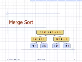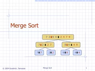
Merge Sort
7 2 9 4 2 4 7 9. 7 2 2 7. 9 4 4 9. 7 7. 2 2. 9 9. 4 4. Merge Sort. Outline and Reading. Divide-and-conquer paradigm (§4.1.1) Merge-sort (§4.1.1) Algorithm Merging two sorted sequences Merge-sort tree Execution example Analysis

Merge Sort
E N D
Presentation Transcript
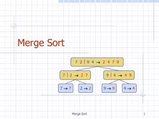
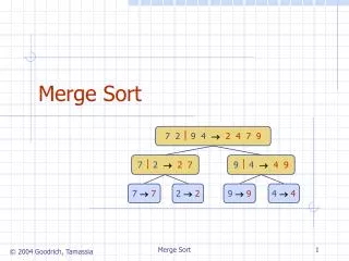
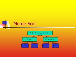
7 2 9 4 2 4 7 9 7 2 2 7 9 4 4 9 7 7 2 2 9 9 4 4 Merge Sort
Outline and Reading • Divide-and-conquer paradigm (§4.1.1) • Merge-sort (§4.1.1) • Algorithm • Merging two sorted sequences • Merge-sort tree • Execution example • Analysis • Generic merging and set operations (§4.2.1) • Summary of sorting algorithms (§4.2.1)
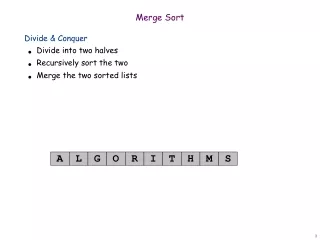
Divide-and conquer is a general algorithm design paradigm: Divide: divide the input data S in two disjoint subsets S1and S2 Recur: solve the subproblems associated with S1and S2 Conquer: combine the solutions for S1and S2 into a solution for S The base case for the recursion are subproblems of size 0 or 1 Merge-sort is a sorting algorithm based on the divide-and-conquer paradigm Like heap-sort It uses a comparator It has O(n log n) running time Unlike heap-sort It does not use an auxiliary priority queue It accesses data in a sequential manner (suitable to sort data on a disk) Divide-and-Conquer
Merge-sort on an input sequence S with n elements consists of three steps: Divide: partition S into two sequences S1and S2 of about n/2 elements each Recur: recursively sort S1and S2 Conquer: merge S1and S2 into a unique sorted sequence Merge-Sort AlgorithmmergeSort(S, C) Inputsequence S with n elements, comparator C Outputsequence S sorted • according to C ifS.size() > 1 (S1, S2)partition(S, n/2) mergeSort(S1, C) mergeSort(S2, C) Smerge(S1, S2)
Merging Two Sorted Sequences • The conquer step of merge-sort consists of merging two sorted sequences A and B into a sorted sequence S containing the union of the elements of A and B • Merging two sorted sequences, each with n/2 elements and implemented by means of a doubly linked list, takes O(n) time Algorithmmerge(A, B) Inputsequences A and B withn/2 elements each Outputsorted sequence of A B S empty sequence whileA.isEmpty() B.isEmpty() ifA.first().element()<B.first().element() S.insertLast(A.remove(A.first())) else S.insertLast(B.remove(B.first())) whileA.isEmpty() S.insertLast(A.remove(A.first())) whileB.isEmpty() S.insertLast(B.remove(B.first())) return S
7 2 9 4 2 4 7 9 7 2 2 7 9 4 4 9 7 7 2 2 9 9 4 4 Merge-Sort Tree • An execution of merge-sort is depicted by a binary tree • each node represents a recursive call of merge-sort and stores • unsorted sequence before the execution and its partition • sorted sequence at the end of the execution • the root is the initial call • the leaves are calls on subsequences of size 0 or 1
7 2 9 4 2 4 7 9 3 8 6 1 1 3 8 6 7 2 2 7 9 4 4 9 3 8 3 8 6 1 1 6 7 7 2 2 9 9 4 4 3 3 8 8 6 6 1 1 Execution Example • Partition 7 2 9 4 3 8 6 11 2 3 4 6 7 8 9
7 2 2 7 9 4 4 9 3 8 3 8 6 1 1 6 7 7 2 2 9 9 4 4 3 3 8 8 6 6 1 1 Execution Example (cont.) • Recursive call, partition 7 2 9 4 3 8 6 11 2 3 4 6 7 8 9 7 2 9 4 2 4 7 9 3 8 6 1 1 3 8 6
7 7 2 2 9 9 4 4 3 3 8 8 6 6 1 1 Execution Example (cont.) • Recursive call, partition 7 2 9 4 3 8 6 11 2 3 4 6 7 8 9 7 2 9 4 2 4 7 9 3 8 6 1 1 3 8 6 7 2 2 7 9 4 4 9 3 8 3 8 6 1 1 6
7 2 2 7 9 4 4 9 3 8 3 8 6 1 1 6 Execution Example (cont.) • Recursive call, base case 7 2 9 4 3 8 6 11 2 3 4 6 7 8 9 7 2 9 4 2 4 7 9 3 8 6 1 1 3 8 6 77 2 2 9 9 4 4 3 3 8 8 6 6 1 1
Execution Example (cont.) • Recursive call, base case 7 2 9 4 3 8 6 11 2 3 4 6 7 8 9 7 2 9 4 2 4 7 9 3 8 6 1 1 3 8 6 7 2 2 7 9 4 4 9 3 8 3 8 6 1 1 6 77 22 9 9 4 4 3 3 8 8 6 6 1 1
Execution Example (cont.) • Merge 7 2 9 4 3 8 6 11 2 3 4 6 7 8 9 7 2 9 4 2 4 7 9 3 8 6 1 1 3 8 6 7 22 7 9 4 4 9 3 8 3 8 6 1 1 6 77 22 9 9 4 4 3 3 8 8 6 6 1 1
Execution Example (cont.) • Recursive call, …, base case, merge 7 2 9 4 3 8 6 11 2 3 4 6 7 8 9 7 2 9 4 2 4 7 9 3 8 6 1 1 3 8 6 7 22 7 9 4 4 9 3 8 3 8 6 1 1 6 77 22 9 9 4 4 3 3 8 8 6 6 1 1
Execution Example (cont.) • Merge 7 2 9 4 3 8 6 11 2 3 4 6 7 8 9 7 2 9 42 4 7 9 3 8 6 1 1 3 8 6 7 22 7 9 4 4 9 3 8 3 8 6 1 1 6 77 22 9 9 4 4 3 3 8 8 6 6 1 1
Execution Example (cont.) • Recursive call, …, merge, merge 7 2 9 4 3 8 6 11 2 3 4 6 7 8 9 7 2 9 42 4 7 9 3 8 6 1 1 3 6 8 7 22 7 9 4 4 9 3 8 3 8 6 1 1 6 77 22 9 9 4 4 33 88 66 11
Execution Example (cont.) • Merge 7 2 9 4 3 8 6 11 2 3 4 6 7 8 9 7 2 9 42 4 7 9 3 8 6 1 1 3 6 8 7 22 7 9 4 4 9 3 8 3 8 6 1 1 6 77 22 9 9 4 4 33 88 66 11
Analysis of Merge-Sort • The height h of the merge-sort tree is O(log n) • at each recursive call we divide in half the sequence, • The overall amount or work done at the nodes of depth i is O(n) • we partition and merge 2i sequences of size n/2i • we make 2i+1 recursive calls • Thus, the total running time of merge-sort is O(n log n)
7 4 9 6 2 2 4 6 7 9 4 2 2 4 7 9 7 9 2 2 9 9 Quick-Sort
Outline and Reading • Quick-sort (§4.3) • Algorithm • Partition step • Quick-sort tree • Execution example • Analysis of quick-sort (4.3.1) • In-place quick-sort (§4.8) • Summary of sorting algorithms
Quick-sort is a randomized sorting algorithm based on the divide-and-conquer paradigm: Divide: pick a random element x (called pivot) and partition S into L elements less than x E elements equal x G elements greater than x Recur: sort L and G Conquer: join L, Eand G Quick-Sort x x L G E x
Partition • We partition an input sequence as follows: • We remove, in turn, each element y from S and • We insert y into L, Eor G,depending on the result of the comparison with the pivot x • Each insertion and removal is at the beginning or at the end of a sequence, and hence takes O(1) time • Thus, the partition step of quick-sort takes O(n) time Algorithmpartition(S,p) Inputsequence S, position p of pivot Outputsubsequences L,E, G of the elements of S less than, equal to, or greater than the pivot, resp. L,E, G empty sequences x S.remove(p) whileS.isEmpty() y S.remove(S.first()) ify<x L.insertLast(y) else if y=x E.insertLast(y) else{ y > x } G.insertLast(y) return L,E, G
7 4 9 6 2 2 4 6 7 9 4 2 2 4 7 9 7 9 2 2 9 9 Quick-Sort Tree • An execution of quick-sort is depicted by a binary tree • Each node represents a recursive call of quick-sort and stores • Unsorted sequence before the execution and its pivot • Sorted sequence at the end of the execution • The root is the initial call • The leaves are calls on subsequences of size 0 or 1
Execution Example • Pivot selection 7 2 9 4 3 7 6 11 2 3 4 6 7 8 9 7 2 9 4 2 4 7 9 3 8 6 1 1 3 8 6 9 4 4 9 3 3 8 8 2 2 9 9 4 4
Execution Example (cont.) • Partition, recursive call, pivot selection 7 2 9 4 3 7 6 11 2 3 4 6 7 8 9 2 4 3 1 2 4 7 9 3 8 6 1 1 3 8 6 9 4 4 9 3 3 8 8 2 2 9 9 4 4
Execution Example (cont.) • Partition, recursive call, base case 7 2 9 4 3 7 6 11 2 3 4 6 7 8 9 2 4 3 1 2 4 7 3 8 6 1 1 3 8 6 11 9 4 4 9 3 3 8 8 9 9 4 4
Execution Example (cont.) • Recursive call, …, base case, join 7 2 9 4 3 7 6 11 2 3 4 6 7 8 9 2 4 3 1 1 2 3 4 3 8 6 1 1 3 8 6 11 4 334 3 3 8 8 9 9 44
Execution Example (cont.) • Recursive call, pivot selection 7 2 9 4 3 7 6 11 2 3 4 6 7 8 9 2 4 3 1 1 2 3 4 7 9 7 1 1 3 8 6 11 4 334 8 8 9 9 9 9 44
Execution Example (cont.) • Partition, …, recursive call, base case 7 2 9 4 3 7 6 11 2 3 4 6 7 8 9 2 4 3 1 1 2 3 4 7 9 7 1 1 3 8 6 11 4 334 8 8 99 9 9 44
Execution Example (cont.) • Join, join 7 2 9 4 3 7 6 1 1 2 3 4 67 7 9 2 4 3 1 1 2 3 4 7 9 7 1779 11 4 334 8 8 99 9 9 44
Worst-case Running Time • The worst case for quick-sort occurs when the pivot is the unique minimum or maximum element • One of L and G has size n - 1 and the other has size 0 • The running time is proportional to the sum n+ (n- 1) + … + 2 + 1 • Thus, the worst-case running time of quick-sort is O(n2) …
Consider a recursive call of quick-sort on a sequence of size s Good call: the sizes of L and G are each less than 3s/4 Bad call: one of L and G has size greater than 3s/4 A call is good with probability 1/2 1/2 of the possible pivots cause good calls: 1 2 3 4 5 6 7 8 9 10 11 12 13 14 15 16 Expected Running Time 7 2 9 4 3 7 6 1 9 7 2 9 4 3 7 6 1 1 7 2 9 4 3 7 6 2 4 3 1 7 9 7 1 1 Good call Bad call Bad pivots Good pivots Bad pivots
Probabilistic Fact: The expected number of coin tosses required in order to get k heads is 2k For a node of depth i, we expect i/2 ancestors are good calls The size of the input sequence for the current call is at most (3/4)i/2n Expected Running Time, Part 2 • Therefore, we have • For a node of depth 2log4/3n, the expected input size is one • The expected height of the quick-sort tree is O(log n) • The amount or work done at the nodes of the same depth is O(n) • Thus, the expected running time of quick-sort is O(n log n)
In-Place Quick-Sort • Quick-sort can be implemented to run in-place • In the partition step, we use replace operations to rearrange the elements of the input sequence such that • the elements less than the pivot have rank less than h • the elements equal to the pivot have rank between h and k • the elements greater than the pivot have rank greater than k • The recursive calls consider • elements with rank less than h • elements with rank greater than k AlgorithminPlaceQuickSort(S,l,r) Inputsequence S, ranks l and r Output sequence S with the elements of rank between l and rrearranged in increasing order ifl r return i a random integer between l and r x S.elemAtRank(i) (h,k) inPlacePartition(x) inPlaceQuickSort(S,l,h - 1) inPlaceQuickSort(S,k + 1,r)
In-Place Partitioning • Perform the partition using two indices to split S into L and E U G (a similar method can split E U G into E and G). • Repeat until j and k cross: • Scan j to the right until finding an element > x. • Scan k to the left until finding an element < x. • Swap elements at indices j and k j k (pivot = 6) 3 2 5 1 0 7 3 5 9 2 7 9 8 9 7 6 9 j k 3 2 5 1 0 7 3 5 9 2 7 9 8 9 7 6 9
Quicksort Speedup • Reduce recursion overhead • Lots of recursive calls for lists of size 1,2,3, etc. How to reduce overhead? • If the size of the list is small (e.g. <=15) use Insertion Sort • How does this affect worst-case runtime? • It doesn’t. O(n2) is constant when n<=15. • Can we sort faster than Ω(n log n) ?
Many sorting algorithms are comparison based. They sort by making comparisons between pairs of objects Examples: bubble-sort, selection-sort, insertion-sort, heap-sort, merge-sort, quick-sort, ... Let us therefore derive a lower bound on the running time of any algorithm that uses comparisons to sort n elements, x1, x2, …, xn. Is xi < xj? no yes Comparison-Based Sorting (§ 4.4)
Let us just count comparisons then. Each possible run of the algorithm corresponds to a root-to-leaf path in a decision tree Counting Comparisons
Decision Tree Height • The height of this decision tree is a lower bound on the running time • Every possible input permutation must lead to a separate leaf output. • If not, some input …4…5… would have same output ordering as …5…4…, which would be wrong. • Since there are n!=1*2*…*n leaves, the height is at least log (n!)
The Lower Bound • Any comparison-based sorting algorithms takes at least log (n!) time • Therefore, any such algorithm takes time at least • Thus, any comparison-based sorting algorithm must run in Ω(n log n) time.
Bucket-Sort and Radix-Sort 1, c 3, a 3, b 7, d 7, g 7, e 0 1 2 3 4 5 6 7 8 9 B
Let be S be a sequence of n (key, element) items with keys in the range [0, N- 1] Bucket-sort uses the keys as indices into an auxiliary array B of sequences (buckets) Phase 1: Empty sequence S by moving each item (k, o) into its bucket B[k] Phase 2: For i = 0, …,N -1, move the items of bucket B[i] to the end of sequence S Analysis: Phase 1 takes O(n) time Phase 2 takes O(n+ N) time Bucket-sort takes O(n+ N) time Bucket-Sort (§ 4.5.1) AlgorithmbucketSort(S,N) Inputsequence S of (key, element) items with keys in the range [0, N- 1]Outputsequence S sorted by increasing keys B array of N empty sequences whileS.isEmpty() f S.first() (k, o) S.remove(f) B[k].insertLast((k, o)) for i 0 toN -1 whileB[i].isEmpty() f B[i].first() (k, o) B[i].remove(f) S.insertLast((k, o))
7, d 1, c 3, a 7, g 3, b 7, e Phase 1 1, c 3, a 3, b 7, d 7, g 7, e B 0 1 2 3 4 5 6 7 8 9 Phase 2 1, c 3, a 3, b 7, d 7, g 7, e Example • Key range [0, 9]
Key-type Property The keys are used as indices into an array and cannot be arbitrary objects No external comparator Stable Sort Property The relative order of any two items with the same key is preserved after the execution of the algorithm Extensions Integer keys in the range [a, b] Put item (k, o) into bucketB[k - a] String keys from a set D of possible strings, where D has constant size (e.g., names of the 50 U.S. states) Sort D and compute the rank r(k)of each string k of D in the sorted sequence Put item (k, o) into bucket B[r(k)] Properties and Extensions
Lexicographic Order • A d-tuple is a sequence of d keys (k1, k2, …, kd), where key ki is said to be the i-th dimension of the tuple • Example: • The Cartesian coordinates of a point in space are a 3-tuple • The lexicographic order of two d-tuples is recursively defined as follows (x1, x2, …, xd) < (y1, y2, …, yd)x1 <y1 x1=y1 (x2, …, xd) < (y2, …, yd) I.e., the tuples are compared by the first dimension, then by the second dimension, etc.
Lexicographic-Sort • Let Ci be the comparator that compares two tuples by their i-th dimension • Let stableSort(S, C) be a stable sorting algorithm that uses comparator C • Lexicographic-sort sorts a sequence of d-tuples in lexicographic order by executing d times algorithm stableSort, one per dimension • Lexicographic-sort runs in O(dT(n)) time, where T(n) is the running time of stableSort AlgorithmlexicographicSort(S) Inputsequence S of d-tuplesOutputsequence S sorted in lexicographic order for i ddownto 1 stableSort(S, Ci) Example: (7,4,6) (5,1,5) (2,4,6) (2, 1, 4) (3, 2, 4) (2, 1, 4) (3, 2, 4) (5,1,5) (7,4,6) (2,4,6) (2, 1, 4) (5,1,5) (3, 2, 4) (7,4,6) (2,4,6) (2, 1, 4) (2,4,6) (3, 2, 4) (5,1,5) (7,4,6)
Radix-sort is a specialization of lexicographic-sort that uses bucket-sort as the stable sorting algorithm in each dimension Radix-sort is applicable to tuples where the keys in each dimension i are integers in the range [0, N- 1] Radix-sort runs in time O(d( n+ N)) Radix-Sort (§ 4.5.2) AlgorithmradixSort(S, N) Inputsequence S of d-tuples such that (0, …, 0) (x1, …, xd) and (x1, …, xd) (N- 1, …, N- 1) for each tuple (x1, …, xd) in SOutputsequence S sorted in lexicographic order for i ddownto 1 bucketSort(S, N)