Chapter 5 - Externalities

1. 1 Chapter 5 - Externalities Public Finance

2. 2 Externality Defined An externality is present when the activity of one entity (person or firm) directly affects the welfare of another entity in a way that is outside the market mechanism. Negative externality: These activities impose damages on others. Positive externality: These activities benefits on others.

3. 3 Nature of Externalities Arise because there is no market price attached to the activity. Can be produced by people or firms. Can be positive or negative. Public goods are special case. Positive externality�s full effects are felt by everyone in the economy.

4. 4 Examples of Externalities Negative Externalities Pollution Cell phones in a movie theater Congestion on the internet Drinking and driving Student cheating that changes the grade curve Positive Externalities Research & development Vaccinations A neighbor�s nice landscape Students asking good questions in class Not Considered Externalities Land prices rising in urban area. Known as �pecuniary� externalities.

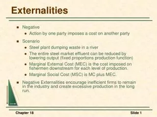
5. 5 Graphical Analysis: Negative Externalities For simplicity, assume that a steel firm owned by Bart dumps pollution into a river that harms a fishery (owned by Lisa) downstream. Competitive markets, firms maximize profits Note that steel firm only care�s about its own profits, not the fishery�s Fishery only cares about its profits, not the steel firm�s.

6. 6 Graphical Analysis, continued MB = marginal benefit to steel firm MPC = marginal private cost to steel firm MD = marginal damage to fishery MSC = MPC+MD = marginal social cost

7. Figure 5.1

8. 8 Graphical Analysis, continued From figure 5.1, as usual, the steel firm maximizes profits at MB=MPC. This quantity is denoted as Q1 in the figure. Social welfare is maximized at MB=MSC, which is denoted as Q* in the figure.

9. 9 Graphical Analysis, Implications Result 1: Q1>Q* Steel firm privately produces �too much� steel, because it does not account for the damages to the fishery. Result 2: Fishery�s preferred amount is 0. Fishery�s damages are minimized at MD=0. Result 3: Q* is not the preferred quantity for either party, but is the best compromise between fishery and steel firm. Result 4: Socially efficient level entails some pollution. Zero pollution is not socially desirable.

10. Figure 5.2

11. 11 Graphical Analysis, Intuition In Figure 5.2, loss to steel firm of moving to Q* is shaded triangle dcg. This is the area between the MB and MPC curve going from Q1 to Q*. Fishery gains by an amount abfe. This is the area under the MD curve going from Q1 to Q*. By construction, this equals area cdhg. Difference between fishery�s gain and steel firm�s loss is the efficiency loss from producing Q1 instead of Q*.

12. 12 Numerical Example: Negative Externalities Assume the steel firm faces the following MB and MPC curves:

13. 13 Numerical Example, continued The steel firm therefore chooses Q1:

14. 14 Numerical Example, continued The deadweight loss of steel firm choosing Q1=140 is calculated as the triangle between the MB and MSC curves from Q1 to Q*.

15. 15 Numerical Example, continued By moving to Q* the steel firm loses profits equal to the triangle between the MB and MPC curve from Q1 to Q* (area cdg).

16. 16 Calculating gains & losses raises practical questions What activities produce pollutants? With acid rain it is not known how much is associated with factory production versus natural activities like plant decay. Which pollutants do harm? Pinpointing a pollutant�s effect is difficult. Some studies show very limited damage from acid rain. What is the value of the damage done? Difficult to value because pollution not bought/sold in market. Possible inference: Housing values may capitalize in pollution�s effect. People may consider neighborhood qualities when buying houses. (ie. Paper mill in backyard)

17. 17 Reflections on these results� We� ve seen how to generate efficiency in the case of externalities. From a practical perspective, computing marginal damages of a pollutant would require economists, engineers, biologists�. Is it ever possible to achieve efficiency without interference? That is, can markets ever find ways to generate efficient outcomes on their own?

18. 18 Private responses There are ways that private individuals, acting on their own, can achieve efficiency in the absence of government. Coase theorem Mergers Social conventions

19. 19 Coase Theorem Insight: root of the inefficiencies from externalities is the absence of property rights. The Coase Theorem states that once property rights are established and transaction costs are small, then one of the parties will bribe the other to attain the socially efficient quantity. The socially efficient quantity is attained regardless of whom the property rights were initially assigned.

20. 20 Illustration of the Coase Theorem Recall the steel firm / fishery example. If the steel firm was assigned property rights, it would initially produce Q1, which maximizes its profits. If the fishery was assigned property rights, it would initially mandate zero production, which minimizes its damages.

21. Figure 5.3

22. 22 Coase Theorem � assign property rights to steel firm Consider the effects of the steel firm reducing production in the direction of the socially efficient level, Q*. This entails a cost to the steel firm and a benefit to the fishery: The steel firm (and its customers) would lose surplus between the MB and MPC curves between Q1 and Q1-1, while the fishery�s damages are reduced by the area under the MD curve between Q1 and Q1-1. Note that the marginal loss in profits is extremely small, because the steel firm was profit maximizing, while the reduction in damages to the fishery is substantial. A bribe from the fishery to the steel firm could therefore make all parties better off.

23. 23 Coase Theorem � assign property rights to steel firm When would the process of bribes (and pollution reduction) stop? When the parties no longer find it beneficial to bribe. The fishery will not offer a bribe larger than it�s MD for a given quantity, and the steel firm will not accept a bribe smaller than its loss in profits (MB-MPC) for a given quantity. Thus, the quantity where MD=(MB-MPC) will be where the parties stop bribing and reducing output. Rearranging, MC+MPC=MB, or MSC=MB, which is equal at Q*, the socially efficient level.

24. 24 Coase Theorem � assign property rights to fishery Similar reasoning follows when the fishery has property rights, and initially allows zero production. The fishery�s damages are increased by the area under the MD curve by moving from 0 to 1. On the other hand, the steel firm�s surplus is increased. The increase in damages to the fishery is initially very small, while the gain in surplus to the steel firm is large. A bribe from the steel firm to the fishery could therefore make all parties better off.

25. 25 Coase Theorem � assign property rights to fishery When would the process of bribes now stop? Again, when the parties no longer find it beneficial to bribe. The fishery will not accept a bribe smaller than it�s MD for a given quantity, and the steel firm will not offer a bribe larger than its gain in profits (MB-MPC) for a given quantity. Again, the quantity where MD=(MB-MPC) will be where the parties stop bribing and reducing output. This still occurs at Q*.

26. 26 When is the Coase Theorem relevant or not? Low transaction costs Few parties involved Source of externality well defined Example: Several firms with pollution Not relevant with high transaction costs or ill-defined externality Example: Air pollution

27. 27 Private responses, continued Mergers Social conventions

28. 28 Mergers Mergers between firms �internalize� the externality. A firm that consisted of both the steel firm & fishery would only care about maximizing the joint profits of the two firms, not either�s profits individually. Thus, it would take into account the effects of increased steel production on the fishery.

29. 29 Social Conventions Certain social conventions can be viewed as attempts to force people to account for the externalities they generate. Examples include conventions about not littering, not talking in a movie theatre, etc. Obviously, here people must be willing to cooperate with social conventions, even though there may be no personal incentive to do so.

30. 30 Public responses Taxes Subsidies Creating a market Regulation

31. 31 Taxes Again, return to the steel firm / fishery example. Steel firm produces inefficiently because the prices for inputs incorrectly signal social costs. Input prices are too low. Natural solution is to levy a tax on a polluter. A Pigouvian tax is a tax levied on each unit of a polluter�s output in an amount just equal to the marginal damage it inflicts at the efficient level of output.

32. Figure 5.4

33. 33 Taxes This tax clearly raises the cost to the steel firm and will result in a reduction of output. Will it achieve a reduction to Q*? With the tax, t, the steel firm chooses quantity such that MB=MPC+t. When the tax is set to equal the MD evaluated at Q*, the expression becomes MB=MPC+MD(Q*). Graphically it is clear that MB(Q*)-MPC(Q*)=MD(Q*), thus the firm produces the efficient level.

34. 34 Numerical Example: Pigouvian taxes Returning to the numerical example:

35. 35 Numerical Example: Pigouvian taxes Setting t=MD(60) gives t=160. The firm now sets MB=MPC+t, which then yields Q*.

36. 36 Public responses Subsidies Creating a market Regulation

37. 37 Subsidies Another solutions is paying the polluter to not pollute. Assume this subsidy was again equal to the marginal damage at the socially efficient level. Steel firm would cut back production until the loss in profit was equal to the subsidy; this again occurs at Q*. Subsidy could induce new firms to enter the market, however.

38. 38 Public responses Creating a market Regulation

39. 39 Creating a market Sell producers permits to pollute. Creates market that would not have emerged. Process: Government sells permits to pollute in the quantity Z*. Firms bid for the right to own these permits, fee charged clears the market. In effect, supply of permits is inelastic.

40. Figure 5.6

41. 41 Creating a market, continued Process would also work if the government initially assigned permits to firms, and then allowed firms to sell permits. Distributional consequences are different � firms that are assigned permits initially now benefit. One advantage over Pigouvian taxes: permit scheme reduces uncertainty over ultimate level of pollution when costs of MB, MPC, and MD are unknown.

42. 42 Public responses Regulation

43. 43 Regulation Each polluter must reduce pollution by a certain amount or face legal sanctions. Inefficient when there are multiple firms with different costs to pollution reduction. Efficiency does not require equal reductions in pollution emissions; rather it depends on the shapes of the MB and MPC curves.

44. Figure 5.7

45. 45 The U.S. response 1970�s: Regulation Congress set national air quality standards that were to be met independent of the costs of doing so. 1990�s: Market oriented approaches have somewhat more influence, but not dominant 1990 Clean Air Act created a market to control emissions of sulfur dioxide with permits.

46. 46 Graphical Analysis: Positive Externalities For simplicity, assume that a university conducts research that has spillovers to a private firm. Competitive markets, firms maximize profits Note that university only care�s about its own profits, not the private firm�s. Private firm only cares about its profits, not the university�s.

47. 47 Graphical Analysis, continued MPB = marginal private benefit to university MC = marginal cost to university MEB = marginal external benefit to private firm MSB = MPB+MEB = marginal social benefit

48. Figure 5.8

49. 49 Graphical Analysis, continued From figure 5.8, as usual, the university maximizes profits at MPB=MC. This quantity is denoted as R1 in the figure. Social welfare is maximized at MSB=MC, which is denoted as R* in the figure.

50. 50 Graphical Analysis, Implications Result 1: R1<R* University privately produces �too little� research, because it does not account for the benefits to the private firm. Result 2: Private firm�s preferred amount is where the MEB curve intersects the x-axis. Firm�s benefits are maximized at MEB=0. Result 3: R* is not the preferred quantity for either party, but is the best compromise between university and private firm.

51. 51 Graphical Analysis, Intuition In Figure 5.8, loss to university of moving to R* is the triangle area between the MC and MPB curve going from R1 to R*. Private firm gains by the area under the MEB curve going from R1 to R*. Difference between private firm�s gain and university�s loss is the efficiency loss from producing R1 instead of R*.

52. 52 Recap of externalities Externalities definition Negative externalities � graphical & numerical examples Private responses Public responses Positive externalities