Download

1 / 13
130 likes | 211 Views
William Greene Stern School of Business New York University. Microeconometric Modeling. Bootstrapping and Quantile Regresion. Estimating the Asymptotic Variance of an Estimator. Known form of asymptotic variance: Compute from known results

E N D
William Greene Stern School of Business New York University Microeconometric Modeling
Estimating the Asymptotic Variance of an Estimator • Known form of asymptotic variance: Compute from known results • Unknown form, known generalities about properties: Use bootstrapping • Root N consistency • Sampling conditions amenable to central limit theorems • Compute by resampling mechanism within the sample.
Bootstrapping Method: 1. Estimate parameters using full sample: b 2. Repeat R times: Draw n observations from the n, with replacement Estimate with b(r). 3. Estimate variance with V = (1/R)r [b(r) - b][b(r) - b]’ (Some use mean of replications instead of b. Advocated (without motivation) by original designers of the method.)
Bootstrap Regression - Replications matrix;bboot=init(3,21,0.)$ Store results here namelist;x=one,y,pg$ Define X regress;lhs=g;rhs=x$ Compute and display b calc;r=0$ Counter proc Define procedure regress;quietly;lhs=g;rhs=x$ … Regression (silent) matrix;{r=r+1};bboot(*,r)=b$ ... Store b(r) endproc Ends procedure execute;n=20;bootstrap=b$ 20 bootstrap reps matrix;list;bboot' $ Display replications
Results of Bootstrap Procedure --------+------------------------------------------------------------- Variable| Coefficient Standard Error t-ratio P[|T|>t] Mean of X --------+------------------------------------------------------------- Constant| -79.7535*** 8.67255 -9.196 .0000 Y| .03692*** .00132 28.022 .0000 9232.86 PG| -15.1224*** 1.88034 -8.042 .0000 2.31661 --------+------------------------------------------------------------- Completed 20 bootstrap iterations. ---------------------------------------------------------------------- Results of bootstrap estimation of model. Model has been reestimated 20 times. Means shown below are the means of the bootstrap estimates. Coefficients shown below are the original estimates based on the full sample. bootstrap samples have 36 observations. --------+------------------------------------------------------------- Variable| Coefficient Standard Error b/St.Er. P[|Z|>z] Mean of X --------+------------------------------------------------------------- B001| -79.7535*** 8.35512 -9.545 .0000 -79.5329 B002| .03692*** .00133 27.773 .0000 .03682 B003| -15.1224*** 2.03503 -7.431 .0000 -14.7654 --------+-------------------------------------------------------------
Bootstrap Replications Full sample result Bootstrapped sample results
Quantile Regression • Q(y|x,) = x, = quantile • Estimated by linear programming • Q(y|x,.50) = x, .50 median regression • Median regression estimated by LAD (estimates same parameters as mean regression if symmetric conditional distribution) • Why use quantile (median) regression? • Semiparametric • Robust to some extensions (heteroscedasticity?) • Complete characterization of conditional distribution
Estimated Variance for Quantile Regression • Asymptotic Theory • Bootstrap – an ideal application
= .25 = .50 = .75
OLS vs. Least Absolute Deviations ---------------------------------------------------------------------- Least absolute deviations estimator............... Residuals Sum of squares = 1537.58603 Standard error of e = 6.82594 Fit R-squared = .98284 Adjusted R-squared = .98180 Sum of absolute deviations = 189.3973484 --------+------------------------------------------------------------- Variable| Coefficient Standard Error b/St.Er. P[|Z|>z] Mean of X --------+------------------------------------------------------------- |Covariance matrix based on 50 replications. Constant| -84.0258*** 16.08614 -5.223 .0000 Y| .03784*** .00271 13.952 .0000 9232.86 PG| -17.0990*** 4.37160 -3.911 .0001 2.31661 --------+------------------------------------------------------------- Ordinary least squares regression ............ Residuals Sum of squares = 1472.79834 Standard error of e = 6.68059 Standard errors are based on Fit R-squared = .98356 50 bootstrap replications Adjusted R-squared = .98256 --------+------------------------------------------------------------- Variable| Coefficient Standard Error t-ratio P[|T|>t] Mean of X --------+------------------------------------------------------------- Constant| -79.7535*** 8.67255 -9.196 .0000 Y| .03692*** .00132 28.022 .0000 9232.86 PG| -15.1224*** 1.88034 -8.042 .0000 2.31661 --------+-------------------------------------------------------------