Download
1 / 31
310 likes | 427 Views
Engineering Diffraction: Update and Future Plans. Ersan Üstündag Iowa State University. Engineering Diffraction: Scope. Main objective : Predict lifetime and performance Needed: Accurate in-situ constitutive laws: = f() Measurement of service conditions: residual and internal stress.

E N D
Engineering Diffraction:Update and Future Plans Ersan Üstündag Iowa State University
Engineering Diffraction: Scope • Main objective: Predict lifetime and performance • Needed: • Accurate in-situ constitutive laws: = f() • Measurement of service conditions: residual and internal stress
Incident h1k1l1 Scattered h1k1l1 Incident h2k2l2 Scattered h2k2l2 Engineering Diffraction: Typical Experiment Eng. Diffractometers: SMARTS (LANSCE) ENGIN X (ISIS) VULCAN (SNS) Typical engineering studies: • Deformation studies • Residual stress mapping • Texture analysis • Phase transformations Challenges: • Small strains (~0.1%) • Quick and accurate setup • Efficient experiment design and execution • Realistic pattern simulation • Real time data analysis • Realistic error propagation • Comparison to mechanics models • Microstructure simulation Bragg’s law: = 2dsin
Engineering Diffraction: Vision for DANSE • Objectives: • Enable new science (& enhance the value of EngND output) • Utilize beam time more efficiently • Help enlarge user community • Approach: • Experiment planning and setup: (Task 7.1) • Experiment design • Optimum sample handling (SScanSS) • Error analysis • Mechanics modeling (FEA, SCM): (Task 7.2) • Multiscale (continuum to mesoscale) • Constitutive laws: = f() • Experiment simulation: (Task 7.3) • Instrument simulation (pyre-mcstas) • Microstructure simulation (forward / inverse analysis) • Impact: • Re-definition of diffraction stress analysis • Easy transfer to synchrotron XRD
Engineering Diffraction: Typical Experiment • Proposed Applications • Experiment Design and Simulation • Instrument simulation • Optimization of parameters • Microstructure simulation • Mechanics modeling I: finite element analysis (FEA) • Mechanics modeling II: self-consistent modeling (SCM) • Data analysis Efforts underway in all of these tasks
Experiment Design and Simulation • Instrument simulation • McStas • Machine studies (SMARTS, ENGIN X) • Optimization of parameters • Sample setup and alignment (SScanSS) • Parametric studies (e.g., neural network analysis) • Microstructure simulation • Defining the sample kernel for experiment simulation • Full forward simulation of experiment
ISIS: SScanSS Software • Implemented on ENGIN X • Ideal for efficient sample setup • Controlled by IDL scripts • Generates a computer image of sample • Creates and executes a measurement plan • Performs GSAS analysis • Creates 2-D data/result plots J. James et al.
Experiment Design and Simulation • Instrument characterization (machine studies) SMARTS ENGIN-X
(a) Engineering Diffraction: Microstructure • Si single crystals (0.7 and 20 mm thick) • SMARTS data • Double peaks due to dynamical diffraction
(b) Engineering Diffraction: Microstructure • Si single crystal (20 mm thick) • ENGIN-X depth scan • Data originates from surface layers Critical question: Transition between a single crystal and polycrystal? E. Ustundag et al., Appl. Phys. Lett. (2006)
Object Oriented Finite Element Analysis A. Reid (NIST) • Modeling of real microstructure • Will be employed in DANSE for microstructure modeling • Needs to become 3-D and validated
[111] [001] [111] 0.1 μm 1 μm 5 μm x-dim 5 μm z y x Three Grain Model Description Microstructure Simulation • Unixaxial Tension: σapplied = 100, 200 & 300 MPa (along x) • x-dim varies:5 μm, 3 μm, 1 μm, 0.8 μm, 0.6 μm • Cu parametersC11111 = 220.3 GPa, C11112 = 104.1 GPa, C11144 = 40.8 GPa C00111 = 168.4 GPa, C00112 = 121.4 GPa, C00144 = 75.4 GPa I.C. Noyan et al.
0.1 μm 1 μm Bulk Strain Values Interaction strain we are interested in measuring. 5 μm 3 μm 5 μm z y x Results from FE Model (300 MPa) • Using COMSOL Multiphysics, we obtain the out of plane strain along center line in central grain. I.C. Noyan et al.
~0.05o Individual Peaks Kinematic X-Ray Modeling • Using kinematic diffraction theory, we simulate a rocking curve diffraction pattern. • Total peak shift of ~0.05o from any one edge. I.C. Noyan et al.
Peak Fitting Analysis • Fitting the diffraction peak with multiple Gaussians, it is possible to determine the peak position and breadth at each step of the summation. • A FWHM value does not necessarily predict a unique strain distribution in a specimen. • How to determine strain profiles from peak position and shape? • What happens in the inelastic regime? I.C. Noyan et al.
Mechanics Modeling • Finite element analysis (FEA) • ABAQUS • Optimization of material parameters • Self-consistent modeling (SCM) • EPSC code from LANL • Optimization of material parameters
Mechanics Modeling:FEA (Finite Element Analysis) Laptop SNS Linux cluster (P) NeXus Archive E1, Y1, E2, Y2 Rietveld ABAQUS a1(P), a2(P) 1c, 2c 1(a1), 2(a2) Compare (fmin) & Optimize (E1,Y1…) 1(1), 2(2)
Framework Optimizer ABAQUS CALL Visualizer call services call services Preprocessor Main processor Postprocessor Use Case Diagram for FEA Application
BMG W-BMG composite Example: BMG-W fiber composite • Residual stresses • Compression loading at SMARTS • Experiments on 20% to 80% volume fraction of W • Unit cell finite element model • GSAS output for average elastic strain in W in the longitudinal direction 20% W/BMG 80% W/BMG Reference: B. Clausen et al., Scripta Mater. 49 (2003) p. 123
Voce Power-law Activity Diagram: FEA (Finite Element Analysis) (P) <include> E1, Y1, E2, Y2 <include> ABAQUS experimental data 1c, 2c 1(a1), 2(a2) Compare & Optimize <include> <include> leastsq fmin 1(1), 2(2) Easy utilization of various software components
σ σ θ0 θ1 n=1 n=4 σo σo n=∞ εo ε εo ε Constitutive Laws for W and BMG Voce Power-law σ1 W BMG Input parameters: (σ0)BMG, nBMG, (σ0)W, (σ1)W, (θ0)W, (θ1)Wand T
Neural Network Analysis Sensitivity Studies • Strong influence by parameters: (σ0)BMG, (σ0)W, (σ1)W and (θ0)W • Weak/no influence by parameters: nBMG,(θ1)W and T • Rigorous experiment planning to optimize data collection L. Li et al.
Neural Network Analysis Result • Use of experimental data for inverse analysis • Prediction of ‘optimum’ values of all 7 input parameters • Previous analyses optimized only 3 parameters L. Li et al.
FEA (Finite Element Analysis) Custom (standard) geometries as templates API release planned for 2007
Mechanics Modeling: Self-Consistent Model <include> Reduce NeXus file User <include> EPSC () • In collaboration with C. Tome (LANL) • Parallel modularization of EPSC, VPSC codes and DANSE implementation <include> I(TOF) pyre-mcstas • Self-consistent modeling (SCM) • Estimate of lattice strain (hkl dependent) • Study of deformation mechanisms
Data Analysis • Peak fitting • Rietveld (full-pattern) analysis GSAS, DiffLab • Single peak fitting • Integration of mechanics models to peak fitting • Strain anisotropy analysis • Texture analysis and visualization (MAUD) • Real-time data analysis
Data Analysis: Mechanical Loading of BaTiO3 • Time-of-flight neutron diffraction data from ISIS • Complete diffraction patterns in one setting • Simultaneous measurement of two strain directions • Different data analysis approaches: • Single peak fitting: natural candidate; but some peaks vanish as the corresponding domain is depleted • Rietveld: crystallographic model fit to all peaks; but results are ambiguous • Constrained Rietveld: multi-peak fitting, but accounting for strain anisotropy (rsca); most promising M. Motahari et al. 2006
Strain Anisotropy Analysis • Desirable to perform multi-peak fitting (e.g. via Rietveld analysis) to improve counting statistics. • Question: How to account for strain anisotropy (hkl-dependent) due to elastic constants and inelastic deformation (e.g., domain switching)? • Current approach for cubic crystals (in GSAS): • is called ‘rsca’ and is a refined parameter for some peak profiles. • Works reasonably well in the elastic regime, but not beyond. • Needed: rigorous multi-peak fitting with peak weighting and peak shift dictated by mechanics modeling. Integration of crystallographic and mechanics models
Engineering Diffraction: Team • E. Üstündag‡, S. Y. Lee, S. M. Motahari, G. Tutuncu (ISU) • X. L. Wang‡(SNS) - VULCAN • C. Noyan‡, L. Li, A. Ying(Columbia) – microstructure • M. Daymond‡(Queens U., ISIS) – ENGIN X, SCM • L. Edwards‡ and J. James (Open U., U.K.) - SScanSS • C. Aydiner, B. Clausen‡, D. Brown, M. Bourke(LANSCE) - SMARTS • J. Richardson‡ (IPNS) • P. Dawson (Cornell) – 3-D FEA • H. Ceylan (ISU) - optimization ‡ Member of EngND Executive Committee