Download
1 / 20
220 likes | 512 Views
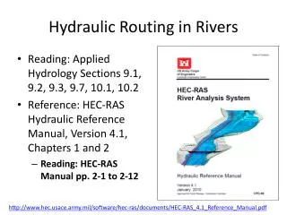
Hydraulic Routing in Rivers. Reference: HEC-RAS Hydraulic Reference Manual, Version 4.1, Chapters 1 and 2 Reading: HEC-RAS Manual pp. 2-1 to 2-12 Applied Hydrology, Sections 10-1 and 10-2. http://www.hec.usace.army.mil/software/hec-ras/documents/HEC-RAS_4.1_Reference_Manual.pdf.

E N D
Hydraulic Routing in Rivers Reference: HEC-RAS Hydraulic Reference Manual, Version 4.1, Chapters 1 and 2 Reading: HEC-RAS Manual pp. 2-1 to 2-12 Applied Hydrology, Sections 10-1 and 10-2 http://www.hec.usace.army.mil/software/hec-ras/documents/HEC-RAS_4.1_Reference_Manual.pdf
One-Dimensional Flow Computations Cross-section Channel centerline and banklines Right Overbank Left Overbank
Flow Conveyance, K Left Overbank Channel Right Overbank
Reach Lengths (1) Floodplain Lch Rob Lob Floodplain (2) Left to Right looking downstream
Solving Steady Flow Equations Q is known throughout reach • All conditions at (1) are known, Q is known • Select h2 • compute Y2, V2, K2, Sf, he • Using energy equation (A), compute h2 • Compare new h2 with the value assumed in Step 2, and repeat until convergence occurs (A) h2 h1 (2) (1)
Flow Computations Reach 3 Reach 2 • Start at the downstream end (for subcritical flow) • Treat each reach separately • Compute h upstream, one cross-section at a time • Use computed h values to delineate the floodplain Reach 1
Unsteady Flow Routing in Open Channels • Flow is one-dimensional • Hydrostatic pressure prevails and vertical accelerations are negligible • Streamline curvature is small. • Bottom slope of the channel is small. • Manning’s equation is used to describe resistance effects • The fluid is incompressible
Continuity Equation Q = inflow to the control volume q = lateral inflow Rate of change of flow with distance Outflow from the C.V. Change in mass Elevation View Reynolds transport theorem Plan View
Momentum Equation • From Newton’s 2nd Law: • Net force = time rate of change of momentum Sum of forces on the C.V. Momentum stored within the C.V Momentum flow across the C. S.
Forces acting on the C.V. • Fg = Gravity force due to weight of water in the C.V. • Ff = friction force due to shear stress along the bottom and sides of the C.V. • Fe = contraction/expansion force due to abrupt changes in the channel cross-section • Fw = wind shear force due to frictional resistance of wind at the water surface • Fp = unbalanced pressure forces due to hydrostatic forces on the left and right hand side of the C.V. and pressure force exerted by banks Elevation View Plan View
Momentum Equation Sum of forces on the C.V. Momentum stored within the C.V Momentum flow across the C. S.
Momentum Equation(2) Local acceleration term Convective acceleration term Pressure force term Gravity force term Friction force term Kinematic Wave Diffusion Wave Dynamic Wave
Momentum Equation (3) Steady, uniform flow Steady, non-uniform flow Unsteady, non-uniform flow
Solving St. Venant equations • Analytical • Solved by integrating partial differential equations • Applicable to only a few special simple cases of kinematic waves • Numerical • Finite difference approximation • Calculations are performed on a grid placed over the (x,t) plane • Flow and water surface elevation are obtained for incremental time and distances along the channel x-t plane for finite differences calculations